Warming

This Web-Project represents an accounting of temperature change that is projected for North America in 2041-2070. Regional Climate Models (RCMs) are run 60 years into the future for small, 50 km x 50 km regions in North America, and their results are analyzed statistically for all regions and all four Boreal seasons. The preponderance of results throughout all of North America is one of warming, usually more than 2°C (3.6°F). A Bayesian, spatial, two-way analysis of variance (ANOVA) model is used to analyze RCM data from the North American Regional Climate Change Assessment Program (NARCCAP).

Introduction

Description of the science problem

Climate models have become primary tools for scientists to project future climate change and to understand its potential impact. Since the late 1960s, Atmosphere-Ocean General Circulation Models (GCMs) have been developed to simulate the climate over the entire globe. GCMs couple an atmospheric model with an oceanic model to simulate components of the global climate system, such as circulations and forcings. Due to model complexity and limitations of computational resources, GCMs are restricted to generate outputs on coarse spatial scales, typically 200 to 500 km. Additionally, due to their global perspective, GCMs usually oversimplify the regional climate processes and geophysical features, such as topography and land cover. Since local/regional climate effects are more relevant to natural-resource management and environmental-policy decisions, Regional Climate Models (RCMs) have been developed to produce high-resolution outputs on scales of 20 to 50 km. Nevertheless, RCMs need initial conditions and time-dependent boundary conditions, which are typically provided by a GCM; this is sometimes referred to as "dynamic downscaling" of the GCM outputs (e.g., Fennessy and Shukla, 2000; Xue et al., 2007).

Essentially, both GCMs and RCMs are a series of discretized differential equations that attempt to represent physical relationships such as the flows of energy and water within and between the atmosphere, oceans, land, sea ice, etc. Using differential equations that describe the physical dynamics, RCMs can simulate 3-hourly "weather" over long time periods and generate a vast array of outputs, from which the long-run average is commonly used as a summary of how a climate model approximates the Earth's climate. With anthropogenic forcings incorporated, climate models can be run under different scenarios (e.g., various CO2 levels), and thus they provide a means to assess natural and anthropogenic influences on climate variability.

GCMs and RCMs are complicated to build and, while any one model is deterministic, their outputs are subject to various sources of uncertainty. For example, uncertainty may be due to complexity of assumptions made about interaction between atmospheric circulation and orography, about discretization, or about parameterizations of the physical-forcing processes. To obtain a better understanding of such uncertainties, climate scientists carry out experiments with multiple runs of multiple models. In this Web-Project, we consider a subset of the climate-model experiment associated with the North American Regional Climate Change Assessment Program (NARCCAP). We propose a statistical framework to summarize the results, which is based on a Bayesian hierarchical spatial analysis of variance (ANOVA) model.

Description of the NARCCAP project

NARCCAP is an international program to produce high-resolution weather and climate simulations in order to investigate spatial variability in regional-scale projections of future climate and to generate temperature-change scenarios for use in impacts research. NARCCAP is designed to investigate the variability in RCMs and provide high-resolution (approximately 50 km) climate-output data for the North American region (Mearns et al., 2009). Phase I explores the variability in RCM outputs for the current period, where six RCMs were run with common boundary conditions provided by the NCEP-DOE Reanalysis II data (e.g., Kanamitsu et al., 2002). NARCCAP Phase II involves not only multiple RCMs, but also runs with different boundary conditions provided by different GCMs. In Phase II, RCMs are run, not only for the current period (1971-2000) but also for a future period (2041-2070), and thus temperature-change projections are available from the Phase II experiment.

Description of the Data used in this Web-Project

A set of six RCMs are included in NARCCAP to produce high-resolution (approximately 50 km) outputs over the spatial domain covering most of Canada, the 48 contiguous states in the United States and northern Mexico, as well as the adjacent Atlantic and Pacific Oceans. In Phase II of NARCCAP, these six RCMs are coupled with a collection of four different GCMs. For each RCM+GCM combination specified in Phase II, two climate-model runs are specified: A current run is implemented from 1971 through 2000; and a future run is implemented from 2041 through 2070, with boundary conditions produced by the same GCMs and with the greenhouse-gas SRES A2 emissions scenario for the 21st century (Nakicenovic et al., 2000).

In this Web-Project, we consider a subset of the Phase II runs whose results are available, and we analyze outputs from two RCMs (with boundary conditions provided by the same GCM in the current period and the future period). In particular, we consider the average surface temperature in the Boreal spring (March, April, and May), Boreal summer (June, July, and August), Boreal autumn (September, October, and November), and Boreal winter (December, January, and February), for the current period (1971-2000) and the future period (2041-2070), produced by two RCMs (CRCM and RCM3) with the same GCM (CGCM3) providing the boundary conditions; for details on these and other climate models used, see Kang and Cressie (2012). The outputs from the RCMs were given on a 50 km x 50 km NARCCAP grid of 98 x 120 points. In all, there are 11,760 NARCCAP gridpoints, times 4 seasons, times 2 RCMs, which results in n=94,080 data that we analyze statistically.

It can be seen from the left panels of Figure 1 that the temperature changes are uniformly positive for all seasons. That is, RCM3 projects that it will be warmer in the future over the entire North American region, no matter the season. We also notice that, generally speaking, the warming effect is stronger over the land compared to that over the ocean. Additionally, the warming effect during the Boreal winter in the northern part of the domain is particularly strong, especially in the Hudson Bay area. For the Boreal winter, it seems that CRCM projects only slightly larger temperature change than does RCM3 (lower-right panel of Figure 1), while it is the opposite in the Boreal summer (second-from-upper-right panel of Figure 1).

It can be seen from the left panels of Figure 1 that the temperature changes are uniformly positive for all seasons. That is, RCM3 projects that it will be warmer in the future over the entire North American region, no matter the season. We also notice that, generally speaking, the warming effect is stronger over the land compared to that over the ocean. Additionally, the warming effect during the Boreal winter in the northern part of the domain is particularly strong, especially in the Hudson Bay area. For the Boreal winter, it seems that CRCM projects only slightly larger temperature change than does RCM3 (lower-right panel of Figure 1), while it is the opposite in the Boreal summer (second-from-upper-right panel of Figure 1).

Figure 1: Left column: Regional temperature-change projections (for RCM3) for four Boreal seasons, spring, summer, autumn, and winter, from the top, down; units are in °C. Right column: Regional temperature-change projection differences for CRCM minus RCM3, for the four Boreal seasons; units are in °C. To avoid distortion, the color scale on the left stops at 5°C , although there are higher temperatures for a few pixels on the maps (max. temperature difference = 7.18°C , in the lower-left panel). [Source: Kang and Cressie (2012)]

Bayesian Spatial Analysis of Variance (ANOVA)

Introduction to bayesian hierarchical modeling

A Bayesian hierarchical model is a type of statistical model where the uncertainty in the parameters is modeled through probability distributions. In many applications, including the one described here, the model can be broken down into three levels: The data model, the process model, and the parameter (or prior) model that, when multiplied together, form the joint distribution of all data, the process, and the parameters (e.g., Berliner, 1996). The data model describes the likelihood of the data, given the parameters and an unobserved (latent) process. The process model describes the probability distribution of the latent process given the parameters. The parameter model puts a "prior" distribution on the parameters themselves, obtained from a priori information.

In the application presented here, which is based on the article by Kang and Cressie (2012), the data model describes the long-run average differences between future and current climate-model runs, where the latent climate process is the projection of temperature change by season and RCM. The process model incorporates the Spatial Random Effects (SRE) model, which is an effective way to reduce the dimensionality of the problem from n = 94,080. Prior distributions (i.e., the parameter models) are assigned to the parameters of the hierarchical statistical model. The ultimate goal is to obtain the posterior distribution, which is the joint distribution of the unknowns (process and parameters) in the model given the observed data. Using Bayes' Theorem, the posterior distribution is proportional to the product of the data, process, and parameter models. Simulation procedures, such as Markov chain Monte Carlo methods, are used here to obtain (an empirical estimate of) the posterior distribution of any part of the process or the parameters. Further details on the data-process-parameter Bayesian framework can be found in Cressie and Wikle (2011) and in the Tutorial on Bayesian Statistics for Geophysicists.

There are several advantages to using a hierarchical statistical approach. First, non-hierarchical models with few parameters generally do not fit the data well, whereas non-hierarchical models with many parameters may fit the observed data well but tend to "over-fit" and may not be useful for predictive purposes. Hierarchical statistical models can often fit the data with few parameters and also do well for predictive purposes. Bayesian hierarchical statistical inference includes straightforward inference at unobserved locations, as well as better uncertainty quantification. The interpretation of the Bayesian posterior credible interval for process and parameter estimates is also more intuitive than that of the confidence interval for frequentist inference.

Spatial statistical modeling using the Spatial Random Effects (SRE) model

The SRE model uses a fixed number of known but not-necessarily-orthogonal (multiresolutional) spatial basis functions, which gives a flexible family of nonstationary covariance functions, results in dimension reduction, and yields optimal spatial predictors whose computations are scalable. By modeling spatial data in a hierarchical manner with a process model that includes the SRE model, the choice is whether to estimate the SRE model's parameters (Cressie and Johannesson, 2008) or to take a Bayesian approach and put a prior distribution on them (Kang and Cressie, 2011). SRE models allow exact computation even when the dataset is massive, change-of-support is straightforward, and it is adept at handling data observed at regular or irregular locations.

Spatial ANOVA

In this Web-Project, we present a spatial two-way ANOVA model in a Bayesian framework that allows a coherent statistical analysis of RCM temperature-change projections from NARCCAP Phase II. The variabilities due to RCMs, Boreal seasons, and their interactions are investigated for any spatial location in North America.

Temperature-change projections in North America

The results given below follow closely the article by Kang and Cressie (2012). In our statistical analysis, we obtain inferences for the temperature-change projections based on posterior distributions. We find that warming effects can differ over areas and seasons substantially: For example, the warming effects are much stronger in the north in winter, and they are stronger in the south in summer. We also find that although the two RCMs produce different outputs, the variability between RCMs is very small, when compared to the projected warming effects. Additionally, from our Bayesian analysis, we are able to obtain both point and interval estimates, and it is possible to investigate various contrasts between factor levels of RCM and season. The multi-way SRE model presented in Kang and Cressie (2012) could also be used for analyzing observations from various instruments on different remote-sensing platforms, where the sizes of the datasets are typically large or even massive.

Results

We first present the posterior means (the optimal predictor under squared-error loss) of the average temperature-change projections, averaged over RCMs and seasons. As seen from the upper-left panel of Figure 2, the posterior means of the average temperature-change projections are above zero (i.e., warming) over the entire spatial domain in North America.

The posterior standard deviations of the average temperature-change projections are plotted in the upper-right panel of Figure 2. Overall, the posterior standard deviations over land are larger than those over water (including oceans, lakes, and bay areas). Our Bayesian analysis enables us to consider the full posterior distribution of the average temperature-change projections, as well as its mean and standard deviation. For example, in the lower-left and lower-right panels of Figure 2, we present maps of the pixelwise posterior 2.5th and 97.5th percentiles of the average temperature-change projections, respectively. Percentiles provide us with a posterior probability interval (i.e, credible interval), in contrast to the point estimation provided by the posterior mean. Specifically, the posterior probability that the average temperature-change projection lies in the interval from the 2.5th percentile to the 97.5th percentile is 0.95, for each pixel in the spatial domain.

The posterior 2.5th percentiles are greater than 2°C (3.6°F) for about two thirds of the pixels in the spatial domain, while the posterior 97.5th percentiles are greater than 2°C for more than three fourths (most of them over the land) of the pixels. The 2°C chosen here is different from the 2°C tolerable threshold defined by the European Union, since the latter is defined as the difference between temperatures of the future and the pre-industrial period (1861-1890). Because the average global temperature of the pre-industrial period is about 0.8°C lower than that of the current period, the maps given in Figure 3 are even more alarming. The regions of North America where the temperature-change projection is estimated to be above 2°C are given in the left panel of Figure 3. A more conservative map, based on the lower limit of the 95% credible interval, shows the locations of those two thirds of North American pixels greater than 2°C, referred to above.

Figure 2: Upper-left panel: The posterior mean of the average temperature-change projections. Upper-right panel: The posterior standard deviation of the average temperature-change projections. Lower panels: Pixelwise posterior 2.5th (lower-left) and 97.5th (lower-right) percentiles of the average temperature-change projections. Units for all panels are in °C. [Source: Kang and Cressie (2012)]

Figure 3: Left panel: Locations (in red) where the posterior mean of the average temperature-change projection is greater than 2°C. Right panel: Locations (in red) where the posterior 2.5th percentile of the average temperature-change projection is greater than 2°C. 

Individual locations

Four locations were chosen, as shown by the triangles in Figure 4, representing pixels in the Hudson Bay, the Great Lakes, the Midwest, and the Rocky Mountains. We then computed and plotted the posterior means of the average temperature-change projection for these four locations, which are shown in Figure 5.

Figure 5 illustrates that the effects of season at the four different locations shown in Figure 4. Figure 5 indicates warming on the order of 3°C for each location, with seasonal warming from 1°C to 6°C for the pixel located in the Hudson Bay.

Figure 4: Selected locations in the Hudson Bay, the Great Lakes, the Midwest, and the Rocky Mountains.


Figure 5: Posterior means of the seasonal temperature-change projection for pixels in the Hudson Bay (upper-left panel), the Great Lakes (upper-right panel), the Midwest (lower-left panel), and the Rocky Mountains (lower-right panel). Black vertical bars represent the 95% credible intervals. Units for all panels are in °C.

 Table 1: Hudson Bay Location (latitude=59.97° N, longitude=87.98° W, elevation=0.00 m)

  All Seasons Spring Summer Autumn Winter
Increase (°F) 5.48 5.51 2.12 3.56 10.74
Increase (°C) 3.05 3.06 1.18 1.98 5.97
Credible Interval (°C) (2.94, 3.15) (2.94, 3.18) (1.07, 1.28) (1.87, 2.08) (5.85, 6.09)

Table 2: Great Lakes Location (latitude=46.39° N, longitude=84.86° W, elevation=225.64 m)

  All Seasons Spring Summer Autumn Winter
Increase (°F) 5.00 4.96 5.16 4.59 5.30
Increase (°C) 2.78 2.76 2.87 2.55 2.95
Credible Interval (°C) (2.59, 2.97) (2.56, 2.95) (2.68, 3.06) (2.36, 2.74) (2.76, 3.14)

Table 3: Midwest Location (latitude=44.17° N, longitude=91.29° W, elevation=276.16 m)

  All Seasons Spring Summer Autumn Winter
Increase (°F) 5.00 4.83 5.52 5.06 4.61
Increase (°C) 2.78 2.68 3.06 2.81 2.56
Credible Interval (°C) (2.57, 2.99) (2.47, 2.90) (2.85, 3.28) (2.60, 3.02) (2.35, 2.77)

Table 4: Rocky Mountain Location (latitude=40.41° N, longitude=107.49° W, elevation=2107.16 m)

  All Seasons Spring Summer Autumn Winter
Increase (°F) 5.09 4.46 6.28 5.46 4.14
Increase (°C) 2.83 2.48 3.49 3.03 2.30
Credible Interval (°C) (2.64, 3.01) (2.29, 2.67) (3.31, 3.68) (2.84, 3.22) (2.11, 2.49)

Tables 1 - 4 show the posterior means of temperature-change projections in degrees Fahrenheit (°F) and Celsius (°C), and the corresponding 95% credible intervals (°C), for the four pixels in the Hudson Bay, the Great Lakes, the Midwest, and the Rocky Mountains. They are shown for all four Boreal seasons - spring, summer, autumn, and winter - as well as for the entire year. At all four locations, the all-seasons 95% credible interval is entirely above 2°C, representing a significant warming beyond the European Union's tolerable threshold.

Discussion

An important and natural extension of the current model is to consider multivariate processes. For example, as well as temperature, RCM outputs for precipitation can be studied simultaneously, as do Sain et al. (2011). More generally, a spatial model could be built by linking RCM outputs to other variables in regional ecosystems, allowing environmental issues, such as water-reservoir capacity, to be addressed. Consequently, statistical inference on quantities used for environmental protection and policy decisions becomes possible.

Finally, we wish to state clearly that our analysis is based solely on the projected temperature change from RCMs, and it cannot detect temperature-change patterns that the RCMs fail to describe. If validation of RCMs is the purpose, then RCM outputs should be compared with actual climate (i.e., a long-term summary of meteorological observations), something NARCCAP Phase I is able to do. However, this is not possible with NARCCAP Phase II, since it involves climate projections into the future. Generally speaking, validation studies to detect (climate) model biases would benefit from a spatial analysis, such as given in this Web-Project.

Acknowledgments

The research presented in this Web-Project was partially supported by NASA's Earth Science Technology Office through its Advanced Information Systems Technology Program and by the Statistical and Applied Mathematical Sciences Institute (SAMSI) in North Carolina. The North American Regional Climate Change Assessment Program (NARCCAP) provided the data used in this Web-Project. NARCCAP is funded by the National Science Foundation (NSF), the U.S. Department of Energy (DoE), the National Oceanic and Atmospheric Administration (NOAA), and the U.S. Environmental Protection Agency (EPA) Office of Research and Development.

Berliner, L.M., 1996. Hierarchical Bayesian time series models, in Maximum Entropy and Bayesian Methods, K. M. Hanson and R. N. Silver (eds.). Kluwer Academic Publishers, Dordrecht, NL, 15-22.

Cressie, N., Johannesson, G., 2008. Fixed rank kriging for very large datasets. Journal of the Royal Statistical Society, Series B 70, 209-226.

Cressie, N., Wikle, C.K., 2011. Statistics for Spatio-Temporal Data. Wiley, Hoboken, NJ.

Fennessy, M.J., Shukla, J., 2000. Seasonal prediction over North America with a regional model nested in a global model. Journal of Climate 13, 2605-2627.

Kanamitsu, M., Ebisuzaki, W., Woollen, J., Yang, S.K., Hnilo, J.J., Fiorino, M., Potter, G.L., 2002. NCEP-DOE AMIP-II Reanalysis (R-2). Bulletin of the American Meteorological Society 83, 1631-1644.

Kang, E.L., Cressie, N., 2011. Bayesian inference for the Spatial Random Effects model. Journal of the American Statistical Association 106, 972-983.

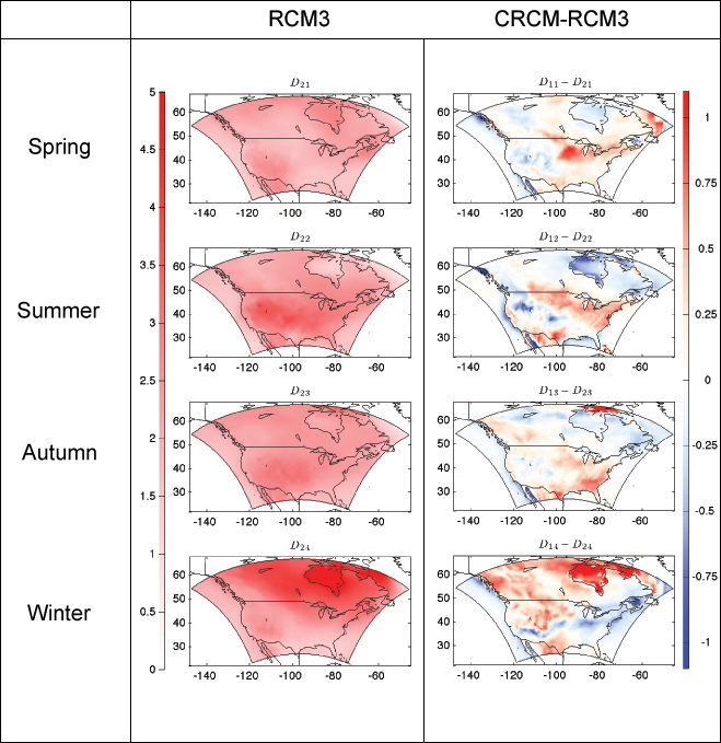
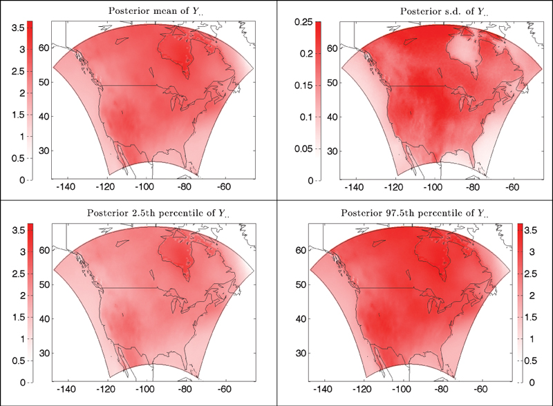
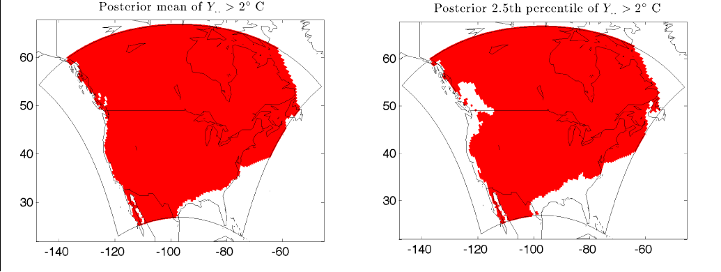
Kang, E.L., Cressie, N., 2012. Bayesian hierarchical ANOVA of regional climate-change projections from NARCCAP Phase II. International Journal of Applied Earth Observation and Geoinformation, in press. doi:10.1016/j.jag.2011.12.007

Mearns, L.O., Gutowski, W.J., Jones, R., Leung, L.Y., McGinnis, S., Nunes, A.M.B., Qian, Y., 2009. A regional climate change assessment program for North America. Eos, Transactions, American Geophysical Union 90, 311-312.

Nakicenovic, N., Alcamo, J., Davis, G., de Vries, B., Fenhann, J., Gaffin, S., Gregory, K., Grubler, A., Jung, T.Y., Kram, T., et al., 2000. Special report on emissions scenarios: A special report of Working Group III of the Intergovernmental Panel on Climate Change. Technical Report. Environmental Molecular Sciences Laboratory, Pacific Northwest National Laboratory, Richland, WA, USA.

Sain, S.R., Furrer, R., Cressie, N., 2011. A spatial analysis of multivariate output from regional climate models. Annals of Applied Statistics 5, 150-175.

Xue, Y., Vasic, R., Janjic, Z., Mesinger, F., Mitchell, K.E., 2007. Assessment of dynamic downscaling of the continental US regional climate using the Eta/SSiB Regional Climate Model. Journal of Climate 20, 4172-4193.