Global mapping of CO2

CO₂

• Global mapping of CO2
• The Global carbon cycle
• Statistical remote sensing
• Spatial analysis of CO2
• Spatio-temporal analysis of CO2
• Combining observations from two instruments: spatio-temporal data fusion
• Datasets and Matlab code
• Acknowledgments
• References
• Links

Global mapping of CO₂

This Web-Project describes spatial and spatio-temporal statistical methodology for mapping CO₂ globally, based on very-large-to-massive remotely sensed datasets.

The global carbon cycle describes where carbon is stored and the movement of carbon between these reservoirs. Atmospheric carbon in the form of carbon dioxide (CO₂) has risen steadily since the industrial revolution (when it was about 280 ppm) to a level of about 400 ppm in 2016​; it was about 315 ppm in 1960. The rate of increase would certainly have been greater had it not been for the uptake of CO₂ by the oceans and vegetation/soil (i.e., sinks). Sources of CO₂ include anthropogenic emissions (e.g., burning coal, oil, or natural gas) and fires. Of the approximately 8 Gt per year that enters the atmosphere, about half is anthropogenic. About 4 Gt stays in the atmosphere, and the other 4 Gt is absorbed roughly equally by the oceans and terrestrial processes. This yearly increase of 4 Gt of atmospheric CO₂ is almost certainly unsustainable in the long term.

Along with water vapor, methane, and other gases, CO₂ traps the sun's energy and warms the earth's surface and lower atmosphere. This global warming will likely lead to very complex changes in our climate. The consequences could be enormous, displacing hundreds of millions of people due to melting ice caps and sea-level rise, highly variable weather events, and a scarcity of potable water due to droughts and melting glaciers.

Mitigation for and adaptation to climate change requires a deep understanding of the drivers of climate. However, atmospheric CO₂'s spatio-temporal cycle is largely unknown at scales where mitigation might be possible. Further, climate models require such knowledge for accurate projections into the future.

Remote sensing is an area of environmental science that is more than building an instrument and putting it in orbit. Hardware is useless without software, and an instrument on a satellite platform is scrap metal without algorithms to process the raw radiances and mapping technologies to give a noise-filtered complete map of the phenomenon being studied. Often, such a map becomes “data,” and these derived data have derived uncertainties associated with them (e.g., spatio-temporal variances and covariances). When remote sensing is put into a rigorous statistical framework, the information content in the raw data increases dramatically. Scientific inferences can be made, and information becomes knowledge. The study of global atmospheric CO2, informed by both data and scientific knowledge, is an important scientific endeavor in which spatial and spatio-temporal statistics can play an important role.

Spatial analysis of CO₂

We begin by describing the spatial-only analysis of large, global datasets of CO₂. The goal of most spatial analyses is to predict the distribution of a process of interest based on a number of observations containing measurement error. Traditional spatial statistics requires inversion of the covariance matrix of the data, which requires on the order of n³ computations when there are n observations in the dataset. This is computationally feasible for n up to a few thousand, but it is not feasible when n is in the tens of thousands and above. In such large-data situations, dimension reduction offers a way forward. We do this here by making use of the Spatial Random Effects (SRE) model (Cressie and Johannesson, 2006, 2008), in which the process of interest is modeled as a linear combination of spatial basis functions plus a fine-scale-variation term. Spatial inference using this geostatistical model, termed Fixed Rank Kriging (FRK) by Cressie and Johannesson (2006, 2008), is then feasible even for very large n (up to a million or more), as long as the number of spatial basis functions (i.e., the number of random effects) is much smaller than the number of observations. From a noisy and incomplete dataset of CO₂, complete global maps of predictions and accompanying standard errors can be obtained:

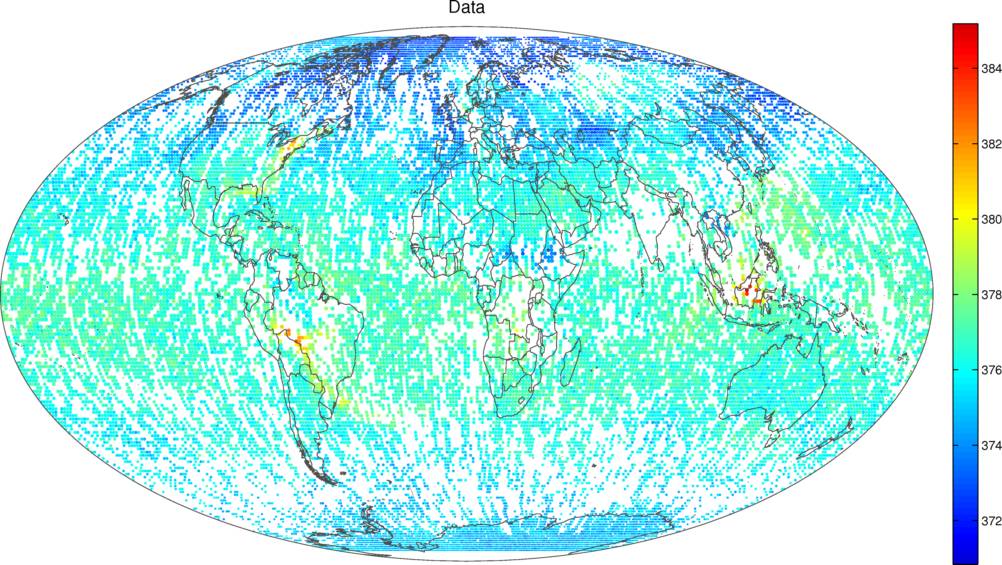
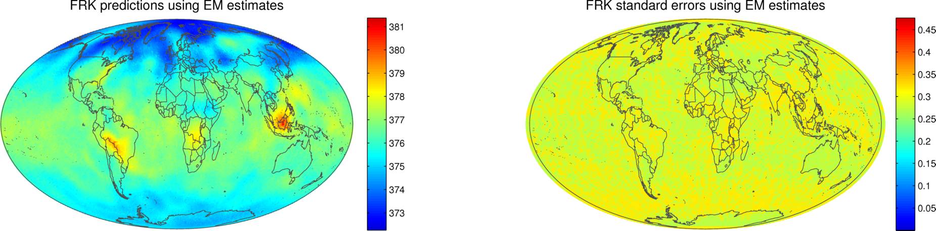
Figure 1: Synthetic (model-based) global CO₂ “measurements” (top) and corresponding FRK predictions and FRK standard errors (using “plug-in” EM estimates). For more details, see the Tutorial on Fixed Rank Kriging (FRK) of CO₂ Data

Parameter estimation or inference can be carried out from an empirical-Bayesian or a fully Bayesian perspective. Cressie and Johannesson (2008) and Kang, Cressie, and Shi (2010) describe binned-method-of-moments parameter estimation, and Katzfuss and Cressie (2009) and Sengupta and Cressie (2013) describe maximum-likelihood estimation via an EM algorithm. These two estimation methods are also described and compared in the Tutorial on Fixed Rank Kriging (FRK) of CO₂ Data.

Bayesian estimation (Kang and Cressie, 2011) provides more accurate uncertainty quantification, but it is also more computationally intensive.

Spatio-temporal analysis of CO₂

We now discuss extensions of the spatial-only statistical methods, given above, to spatio-temporal models. Satellites only cover certain tracks on the globe on any given day, and so the tracks covered on previous days may be highly complementary. We could analyze the data spatially in a sequence of moving windows, which was done for ​Arctic carbon dioxide​​ using a 9-day window and the SRE model. Temporal dependence could be incorporated through a separable temporal covariance function. Alternatively, the (spatio-)temporal dependence in the data can be incorporated statistically by specifying the dynamical evolution of the spatial random effects over time. This is done through a first-order vector autoregressive model (VAR(1)) that is defined by a propagator matrix and an innovations covariance matrix. The resulting spatio-temporal random effects (STRE) model (Cressie, Shi, and Kang, 2010) can then be used to exploit both spatial and temporal dependencies in the process when predicting its distribution at all locations in space and time.

Cressie, Shi, and Kang (2010) called inference in the STRE model Fixed Rank Filtering (FRF) when predictions are made for the current day based on data on the current day and previous days, and Fixed Rank Smoothing (FRS) when predictions are made retrospectively, for a time period of interest, based on all data obtained during the same time period. Again, both empirical-Bayesian inference and fully Bayesian inference are possible. From the empirical-Bayesian perspective, binned-method-of-moments estimation of the parameters of the STRE model is described in Kang, Cressie, and Shi (2010), and EM estimation is described in Katzfuss and Cressie (2011); we refer to this as EM-FRS. Fully Bayesian inference for the STRE model is described in Katzfuss and Cressie (2012); we refer to this as FB-FRS. The prior distribution on the propagator matrix (which describes the temporal evolution of the process on the reduced space) in the latter article can be rather involved; we provide some results there based on the assumption that the propagator matrix is diagonal, but not equal to the identity matrix. The prior there is a special case of the prior in Katzfuss and Cressie (2012), although it still results in complex spatio-temporal dependence.

The Atmospheric InfraRed Sounder (AIRS) on board NASA's Aqua satellite measures spectra from which mid-tropospheric (approximately between altitudes of 2km and 8km) CO₂, at roughly 1:30 pm local time, can be retrieved using elaborate algorithms. The resulting data is provided here and was originally obtained from the AIRS (NASA) website. The unit of measurement is parts per million (ppm).

Figure 2: Spatio-temporal prediction of CO₂ using AIRS data (top): Results from EM-FRS (left) and FB-FRS (right)

Up to this point, we have assumed that only one source of observations is available (e.g., the AIRS instrument). However, more satellite instruments (e.g., the one on board the Japanese GOSAT satellite) capable of retrieving CO₂ are now in operation, and NASA's OCO-2 is under development *. It seems natural to combine the information from these two instruments to obtain better predictions of the true CO₂ field. However, the two instruments have different sensitivities to CO₂ in the atmospheric column, different measurement-error properties, and different footprints, so making predictions based on the data observed by both instruments is not trivial. The general problem of (spatial-only) data fusion is discussed in Nguyen et al. (2012). Nguyen et al. (2014) extends the data-fusion methodology to the spatio-temporal case and applies it to CO₂.

For the spatial-only case, the R-package FRK became available on GitHub in 2016. Matlab code is also available: matlabfunctions.zip contains the Matlab functions FRK.m, EM.m (EM algorithm), variogram_estimation.m (variogram estimation of the fine-scale-variation variance and the measurement-error variance), and binest.m (binned method-of-moments estimation). The file called xco2analysis.m contains code for the analysis of the synthetic CO2 dataset (Figure 1) using these Matlab functions; download the synthetic set of CO2 “measurements.”. For more details, see the Tutorial on Fixed Rank Kriging (FRK) of CO2 Data.

For the spatio-temporal case, the R-package FRK uses a non-dynamical separable spatio-temporal covariance model for prediction. Matlab code is also available: STmatlabfunctions.zip contains the spatio-temporal functions EM_FRS.m (which implements the EM algorithm), and FRS_vxi.m (which implements the FRS procedure, for the case with heterogeneous fine-scale-variation variance). Download the 16 days of AIRS CO2 data used in Figure 2. 

The research was partially supported by NASA under grant NNX08AJ92G issued through the ROSES Carbon Cycle Science Program and grant NNH08ZDA001N issued through the Advanced Information Systems Technology ROSES 2008 Solicitation, by the Office of Naval Research Grant N00014-08-1-0464, and by an Australian Research Council Discovery Grant, number DP150104576.

Notes

* October 2016: NASA's OCO-2 instrument is currently in operation. The OCO-2 satellite launched successfully in July, 2014.

Links

• Tutorial on Fixed Rank Kriging (FRK) of CO₂ Data
• ​AIRS CO₂ data website​​
• ​FRK Package for R​​

This page originally appeared at www.stat.osu.edu/~sses/collab_co2.html. It was updated in October 2016.