Global flux inversion

Global carbon dioxide (CO₂) flux inversion

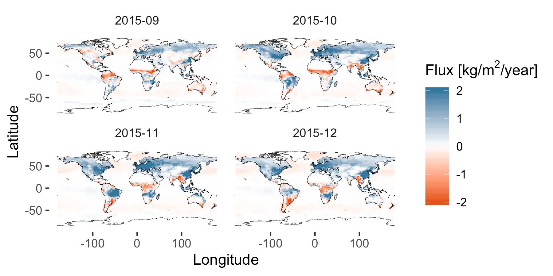
Carbon dioxide (CO₂) flux inversion at the global scale aims to understand the overall pattern in both time and space of all sources and sinks (in one word, fluxes) of CO₂.^[1] Sources and sinks come in many forms, and have different properties. Some are very local, such as power plants, while others are spread out, such as oceanic sources and sinks. Some produce regular and predictable fluxes, such as forests, while others are sporadic and unpredictable, such as forest fires and volcanoes. Many also follow one or more cycles, including night/day (diurnal), weekly, or annual cycles. Importantly, human activity is changing the natural processes that cause the sources and sinks.^[2] Reasons for this include climate change, increases in the amount of CO₂ in the atmosphere, and large-scale changes to the environment such as land usage.^[3,4,5] Improving how well we understand the scale, variability, and space and time patterns of sources and sinks of CO₂ may therefore help people respond to climate change. Figure 1 shows the sort of product this project can produce. It gives an example set of flux maps for September, 2015 through to December, 2015, made using realistic example fluxes.

Figure 1: A flux map for September, 2015 through to December, 2015. The colour of each grid cell shows the average monthly flux in kg/m²/year for that cell. Each panel shows one month of fluxes. The fluxes shown are realistic but were not produced by flux inversion; they are just shown for illustration.

The reason this project is called ‘flux inversion’ instead of ‘flux measurement’ is that most big sources and sinks cannot be measured directly.^[6] Instead, what is seen is the effect of flux on atmospheric CO₂ levels over space and time. The constant movement of the atmosphere means that changes to these levels are not usually seen at the time and location where the flux happened. The only way to find when and where the flux happened is to work backwards from observations. Doing this requires understanding the transport processes that move CO₂ around the globe, and working backwards through this understanding of transport is called inversion.^[6] One of the challenges that comes with flux inversion is that a precise answer is not possible; in mathematical terms, the system is underdetermined. For that reason, uncertainty is very important^[7], and one of our aims in this project is to provide valid statistical measures of uncertainty (otherwise known as uncertainty quantification) for our flux estimates.

The observations of CO₂ levels used for flux inversion come in two forms, in situ and remote sensing. In situ observations are typically made using air samples analysed in laboratories. These may be collected either at fixed facilities, some of which have been operating for decades, or from organised aircraft campaigns. In situ measurements are very precise, but miss many times and locations.^[8] Remote sensing observations are made by satellites using instruments that record how much of the sunlight reflected off the Earth is absorbed by CO₂ molecules. This gives an estimate of how much CO₂ is in the column of air below the satellite. Remote sensing observations are usually less precise than in situ observations, but there are many of them made every day, and they cover a large portion of the globe.^[8,9] This makes remote sensing observations a useful but challenging part of flux inversion, because the high coverage in space and time helps understand patterns of flux, but the high number of observations makes computation difficult. One of the missions measuring CO₂ is NASA’s Orbiting Carbon Observatory 2 (OCO-2) satellite. Figure 2 shows the observations made by OCO-2 from the first two weeks of September, 2015.

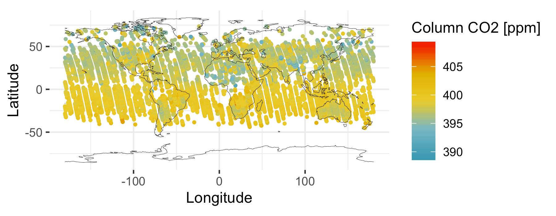
Figure 2: Observations made by the OCO-2 satellite mission for the first two weeks of September, 2015. The colour of the observation shows how much CO₂ was detected as a fraction of the atmosphere in parts-per-million [ppm] in the air below the satellite. The amounts shown are averages of every 10 seconds worth of measurements.

Putting it all together, our project aims to combine three things: the scientific understanding of the transport of CO₂, remote sensing observations, and statistical uncertainty quantification. The result is a Bayesian inversion and computational methodology that allows estimation of statistically justifiable and scientifically important sources and sinks of CO₂, along with uncertainty quantification of those fluxes. The Bayesian global flux inversion framework is known as WOMBAT (WOllongong Methodology for Bayesian Assimilation of Trace-gases); technical details of WOMBAT v1.0 are published in Geoscientific Model Development^[10]. The CEI Web-Project Global CO2 Flux gives a general explanation of the framework. A flux inversion from six years of OCO-2 v10 CO₂ and in situ CO₂ measurements (in ppm) has been implemented using WOMBAT v2.0, and it has been submitted to the OCO-2 v10 Model Intercomparison Project (MIP).  

Authored by M. Bertolacci, 2020.