Global estimation of CO2 sources and sinks (flux) at Earth’s surface is critical for mitigating atmospheric CO2. Flux estimates given in this Web-Project are obtained from atmospheric CO2 concentration data and Bayesian hierarchical statistical models that also yield uncertainties of the estimates.

Global CO2 flux

This Web-Project by Noel Cressie, Josh Jacobson, and Michael Bertolacci, features WOMBAT (the WOllongong Methodology for Bayesian Assimilation of Trace-gases), a framework for estimating fluxes on a global scale. Carbon dioxide (CO2) is one of several greenhouse gases, so-called because they trap heat in Earth’s lower atmosphere. Locations across Earth’s surface where CO2 is added to or removed from the atmosphere are known as sources and sinks – the rate at which this happens is known as flux. The aim of flux inversion is to characterise the pattern and scale of sources and sinks in both space and time. The nature of CO2 sources and sinks can be very different from one location and time point to the next. For example, temperate forests occupy large parts of the terrestrial biosphere and transition from sinks to sources during the year, while volcanoes are local sources with sporadic and unpredictable outgassing of CO2. Human activity has also caused changes to the natural processes that cause these sources and sinks. As a tool to improve our understanding of the scale, variability, and patterns of the sources and sinks of the leading greenhouse gas CO2, WOMBAT produces flux estimates accompanied by uncertainty bounds on the estimates. The framework is designed to help scientists and policy-makers take uncertainty in CO2 flux estimates into account and thus better respond to climate change.

Introduction

Mitigation of global CO2 emissions

In December 2015, 196 countries and territories around the world participated in COP21 in Paris, France and signed an agreement to limit global warming to below 2-degrees Celsius compared to pre-industrial levels. Achieving this target requires a worldwide reduction in greenhouse gas emissions that trap heat near Earth’s surface. Of the greenhouse gases to be controlled, the principal one is carbon dioxide (CO2). Six years later, in November 2021, the parties gathered again for COP26 in Glasgow, Scotland to take stock of progress, and most agreed to enact further commitments to achieve net-zero growth of atmospheric CO2 by 2050.

Figure 1: Global atmospheric carbon dioxide (CO2) concentrations in parts per million (ppm) for the past 800,000 years. Figure from https://www.climate.gov/news-features/climate-qa/doesnt-carbon-dioxide-atmosphere-come-natural-sources.

CO2 is the leading greenhouse gas emitted by human activity, largely as a byproduct of burning fossil fuels. These anthropogenic emissions over the last 200 years have more than doubled the amount of CO2 in the atmosphere. Now, as a result, the human influence on the climate is clear: Figure 1 shows that current CO2 concentrations of more than 400 parts per million (ppm) are greater than anything seen for at least the last 800,000 years.

According to the 2021 IPCC synthesis report, “limiting human-induced global warming to a specific level requires limiting cumulative CO2 emissions, reaching at least net zero CO2 emissions.” This objective is simple to describe, but the actual monitoring and reduction of CO2 emissions is difficult for several reasons. First, humans aren’t the only factor, as plants and animals both emit and absorb CO2 all the time, as does the ocean. Second, the atmosphere is a connected system and the CO2 that is emitted in any one region moves around via weather systems and affects CO2 concentrations across the globe. Mitigating atmospheric CO2 requires an understanding of both of these factors, as well as understanding when and where human activity results in emission of this leading greenhouse gas.

Science problem: global flux inversion

The rate of exchange of CO2 between Earth’s surface and the atmosphere is known as CO2 flux. ​​How the atmosphere responds to CO2 fluxes can be studied using simulations. For example, in Figure 2, we simulate the effect of additional CO2 emissions over parts of North America. The left panel shows a month of added CO2 emissions (flux) in North America, and the right panel is an animation of of the estimated changes in atmospheric-column CO2 concentration (XCO2) showing how the extra CO2 spreads around the globe. By adding together hundreds of such simulated changes in different parts of the globe, we can build a picture of how atmospheric transport works. This animation also illustrates the point made in the previous paragraph, that CO2 emitted in one place moves around the globe—in fact, it moves quite quickly and becomes part of the background CO2 concentration in the hemisphere it is emitted in within a matter of months.

Figure 2

CO2 flux is a key quantity that scientists and policy-makers use to mitigate climate change, but it is usually not possible to measure it directly. It is a rate of change of CO2 over time at every location on Earth’s surface, but a large amount of the flux happens over huge, remote areas, such as Siberia and the Amazon. Instead, the effect of flux, namely CO2 concentration, is measured in parts per million (ppm) of CO2. However, because of atmospheric transport, changes in concentration are not usually seen at the same time or location that the flux happened. To estimate when and where flux has occurred, we need to understand the process that moves CO2 around the globe, called atmospheric transport. Then, in principle, we can work backwards from observations of CO2 concentrations to estimate CO2 fluxes, using a computational-statistical procedure known as flux inversion. Figure 3 shows an example of CO2 concentrations (in ppm) on the left, and the corresponding flux estimates (in kilograms per square metre per year) on the right.

Figure 3: Left panel: CO2 concentration in ppm for a 3-hour period on January 1, 2016. Right panel: Corresponding flux estimates (in kilograms of CO2 per square metre per year) for the previous month, December 2015.

Why solve the problem with Statistics?

Although geophysicists would like to get a perfect estimate of the CO2 fluxes, the complexities of the atmosphere make this impossible. For this reason, any flux estimate should be accompanied by a measure of its uncertainty. The field of Statistics is a mathematical science that quantifies uncertainties in terms of probabilities, and statistical models are the gold standard for doing this.

To carry out flux inversion, we have created a statistical framework called WOMBAT (the WOllongong Methodology for Bayesian Assimilation of Trace-gases; Zammit-Mangion et al., 2022), named after the Australian marsupial shown in Image 1. The WOMBAT framework uses statistical methods to identify and account for different sources of error in the estimates of flux and of concentrations. This will aid scientists and policy-makers in reaching consensus about a stocktake (and ideally mitigation) of the parties’ CO2 emissions since COP21.

The statistical framework WOMBAT is named after the Australian marsupial, pictured here near Cradle Mountain in Tasmania, Australia. Photo by Meg Jerrard.
Image 1: WOMBAT, our statistical framework for flux inversion, is named after the Australian marsupial. ( One is pictured here near Cradle Mountain in Tasmania, Australia. Photo by Meg Jerrard.)

WOMBAT: A fully Bayesian global flux-inversion framework

Image 2: WOMBAT’s CO2 flux-inversion framework consists of a hierarchy of four layers, similar in idea to the hierarchy of Russian nesting dolls. Photo by Didssph on Unsplash.

WOMBAT’s CO2 flux-inversion framework consists of a hierarchy of four layers, similar in idea to the hierarchy of Russian nesting dolls shown in Image 2. The outermost layer, the layer we “see,” is the data itself (call it Z). CO2 concentration can be measured directly in parcels of air collected from the atmosphere, or it can be estimated indirectly from satellites or aircraft measurements (i.e., from remote sensing). But what we see is not generally what we’re after, as each of these measurement techniques is subject to some level of error. This measurement error is accounted for statistically, so that the second layer of WOMBAT’s hierarchy represents the underlying process of CO2 concentrations across the globe (call it Y). Here, a model of the movement (or transport) of CO2 particles through the atmosphere is key to connecting to the third layer, and uncertainty comes from imperfect information about the winds and the physics of atmospheric mixing. The third layer is geophysically the most critical, namely the CO2 fluxes across the globe (call it X). Like many other physical processes, fluxes at times and locations that are close together are more alike than those far apart. WOMBAT models this spatio-temporal dependence statistically in order to obtain valid flux estimates as well as their uncertainties. The fourth and innermost layer of WOMBAT’s hierarchy describes the scientific knowledge and assumptions that inform and control each of the other layers (call it θ). These four layers together define a hierarchy that is connected by statistical models and is shown in Figure 4.

Figure 4: Diagram outlining WOMBAT’s hierarchy of connected layers that incorporate information from remote sensing data, resulting in flux estimates and their uncertainties.

Like an intricate, connected machine, the uncertainty in one layer of the statistical hierarchy can affect the uncertainty and estimates in another layer. To deal with this, the layers are connected using  statistical models and a mathematical result known as Bayes’ Theorem, which shows how different sources of information can be combined in the presence of uncertainty. This statistical framework is called a Bayesian hierarchical model (BHM), and WOMBAT is a geophysical  example of such a model. BHMs appear in many other areas of science.

A technical description of a BHM goes as follows: Let [A] denote the probability distribution of variable A; [A, B] denote the joint probability distribution of the variables A and B; and [A | B] denote the conditional distribution of A given B. Using this notation, the four layers of WOMBAT are connected by the following probability distributions:

            (1) [Z | Y, θ],

            (2) [Y | X, θ],

            (3) [X | θ], and

            (4) [θ].

What distinguishes WOMBAT from other flux inversions is the presence of [θ] and the consequent Markov Chain Monte Carlo (MCMC) sampling needed to obtain [X, Y, θ | Z], which is the posterior distribution of all the hidden variables given the data Z. Estimates of CO2 flux and their uncertainties are obtained from this posterior, specifically from [Y | Z]. For more information, see the Tutorial on Bayesian Statistics for Geophysicists.

Global CO2 flux estimation from WOMBAT

NASA’s OCO-2 satellite data

The data used in this Web-Project come from the Orbiting Carbon Observatory-2 (OCO-2) satellite, NASA’s first remote sensing mission with primary science objective to understand the global geographic distribution of CO2. Data are available dating back to late 2014, a few months after the satellite was launched, and they cover much of each hemisphere, depending on the time of year. Figure 5 shows an example of these data, representing the observations accumulated over the course of one week in January 2016 – notice that the satellite’s orbital path can be seen in the spatial pattern of the observations (OCO-2’s current location is available at the OrbTrack website). The analysis given in this Web-Project follows closely that of Zammit-Mangion et al. (2022), which focuses on OCO-2 data (Version 7) for the two-year period from January 2015 through December 2016.

Figure 5: OCO-2 measurements of atmospheric-column CO2 concentrations (XCO2, in ppm) from 2016-01-01 through 2016-01-07, inclusive.

Monthly estimated fluxes for 2015-2016

The animation shown in Figure 6 gives estimated monthly CO2 fluxes for 2015-01 to 2016-12 across the globe, estimated from WOMBAT and based on two years of OCO-2 satellite data (XCO2 concentrations). Also shown are the uncertainties obtained from WOMBAT. Fossil-fuel fluxes are considered to be well known (at least compared to natural fluxes), so we subtract them from our statistical model and only estimate the natural fluxes. The left panel of the animation shows the map of monthly non-fossil-fuel estimated fluxes (posterior mean in each grid cell) over the globe for each month in (kg/metre squared/second x 1e-7). The right panel shows the map of the corresponding monthly posterior standard deviation in each grid cell (same units), which is a quantification of the uncertainty of the estimated fluxes shown on the left panel.

Figure 6

Notice that the tropics are relatively constant in their flux, while the temperate zones are very seasonal. This seasonal cycle of CO2 is mostly driven by the vast forest areas in the northern hemisphere. Earth is breathing! In autumn and winter, trees drop their leaves, which decompose and release CO2 into the atmosphere; in the spring and summer, leaves grow back and begin drawing down CO2 through the process of photosynthesis; and the cycle repeats. Flux activity over the oceans is less intense at any given time and location, but because oceans cover more than two-thirds of Earth’s surface area, the ocean fluxes are substantial.

Specific flux activity over land and oceans separately can be seen in Figure 7 which shows WOMBAT’s estimates of surface flux -- excluding fossil fuel emissions -- using data from a single satellite mode (Land Glint [LG]). Figure 7 also shows that WOMBAT’s estimates largely agree with flux estimates from the first OCO-2 model intercomparison project (MIP; Crowell et al. 2019). The first row of Figure 7 shows that the combined effects of land and ocean flux lead to Earth’s surface absorbing about 4 petagrams of carbon (PgC) per year on average. Unfortunately, humans are emitting on the order of 10 PgC per year of CO2 into the atmosphere. This addition of approximately 6 PgC per year means that CO2 levels in the atmosphere will only keep increasing, and thus continue to exacerbate climate change.


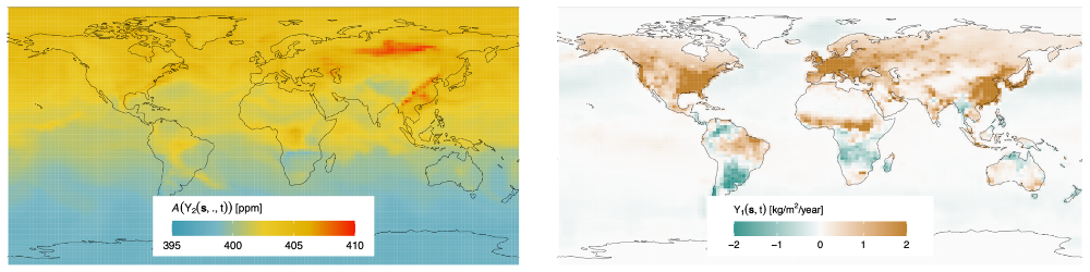
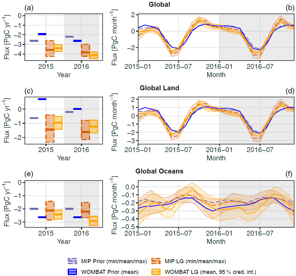
Figure 7: Annual (left column) and monthly (right column) fluxes for the globe (first row), land (second row), and ocean (third row). Summaries of flux estimates from the model intercomparison project (MIP) and the flux estimate from WOMBAT are shown, split into the prior and LG inversions. Figure from Zammit-Mangion et al. (2022).

Conclusions and future work

To control and reduce the build-up of atmospheric CO2 over the next century and uphold the urgent commitments of COP21 and later agreements, it is essential to understand where CO2 is being exchanged with the atmosphere, how these regions vary through time, and whether there are ways to mitigate the sources and enhance the sinks. As a framework for determining where CO2 is emitted and absorbed across Earth’s surface, WOMBAT can aid scientists in the evaluation of CO2 sinks, to understand their long-term viability as well as the possibility of replicating their characteristics in the future over new regions of Earth’s surface. The CO2 flux estimates provided by WOMBAT, together with their statistical uncertainty, give scientists and policy-makers the clarity needed to better mitigate the effect of this leading greenhouse gas, carbon dioxide. 

There are updates and extensions we hope to address in future versions of WOMBAT. For example:

  • Account for remaining uncertainties, particularly in the atmospheric transport model of how CO2 moves around the globe.
  • Carry out flux-inversion for other atmospheric greenhouse gases, such as methane, which are also important to monitor and mitigate.
  • Investigate whether the results presented here could be used to improve smaller-scale, regional or country-scale flux inversions at very high resolutions, such as those of the CarbonWatch-NZ project that estimates fluxes over New Zealand.

Acknowledgements

This Web-Project was supported by Australian Research Council Discovery Project DP190100180 and NASA ROSES grants 17-OCO2-17-0012 and 20-OCOST20-0004.

  • Figure 1: Graph by NOAA via Climate.gov
  • Figure 7: Graph by Zammit-Mangion et al. (2022).
  • Image 1: Photo by Meg Jerrard via Unsplash
  • Image 2: Photo by Didssph via Unsplash