Brown, S. and Heathcote, A. (2008). The simple complete model of choice reaction time: linear ballistic accumulation. Cognitive Psychology, 57, 153-178.
Dao, V. H., Gunawan, D., Brown, S. D., Kohn, R., Tran, M.-N., and Hawkins, G. E. (2023). Bayesian inference for evidence accumulation models with regressors. arXiv preprint arXiv:2302.10389.
Dao, V. H., Gunawan, D., Tran, M.-N., Kohn, R., Hawkins, G. E., and Brown, S. D. (2022). Efficient selection between hierarchical cognitive models: Cross-validation with variational Bayes. Psychological Methods.
Gunawan, D., Carter, C., and Kohn, R. (2023a). The correlated particle hybrid sampler for state space model. arXiv preprint arXiv:1804.04359v4.
Gunawan, D., Chatterjee, P., and Kohn, R. (2023b). The block correlated pseudo marginal method for state space model. arXiv preprint arXiv:2109.14194.
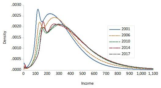
Gunawan, D., Griffiths, W., and Chotikapanich, D. (2022a). Inequality in education: A comparison of Australian indigenous and nonindigenous populations. Statistics, Politics and Policy, 13(1), 57–72.
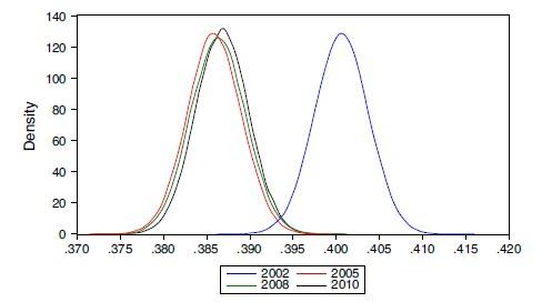
Gunawan, D., Griffiths, W. E., and Chotikapanich, D. (2018). Bayesian inference for health inequality and welfare using qualitative data. Economics Letters, 162, 76–80.
Gunawan, D., Griffiths, W. E., and Chotikapanich, D. (2021a). Posterior probabilities for Lorenz and stochastic dominance of Australian income distributions. Economic Record, 97(319), 504–524.
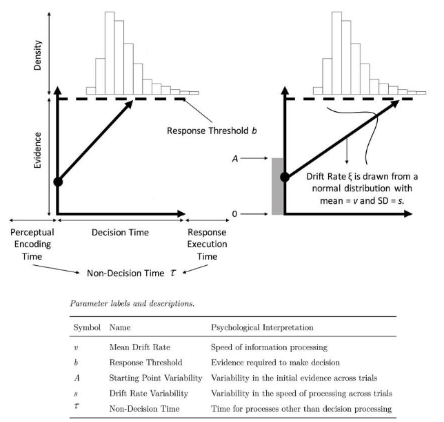
Gunawan, D., Hawkins, G. E., Kohn, R., Tran, M.-N., and Brown, S. D. (2022b). Time-evolving psychological processes over repeated decisions. Psychological review, 129(3), 438.
Gunawan, D., Hawkins, G. E., Tran, M.-N., Kohn, R., and Brown, S. (2020). New estimation approaches for the hierarchical linear ballistic accumulator model. Journal of Mathematical Psychology, 96, 102368.
Gunawan, D., Kohn, R., and Nott, D. (2021b). Variational Bayes approximation of factor stochastic volatility models. International Journal of Forecasting, 37(4), 1355–1375.
Gunawan, D., Kohn, R., and Nott, D. (2023c). Flexible variational Bayes based on a copula of a mixture. Journal of Computational and Graphical Statistics, pages 1–16.
Gunawan, D., Kohn, R., and Tran, M. N. (2022c). Flexible and robust particle tempering for state space models. Econometrics and Statistics.
Lander, D., Gunawan, D., Griffiths, W. E., and Chotikapanich, D. (2020). Bayesian assessment of Lorenz and stochastic dominance. Canadian Journal of Economics.
Mendes, E. F., Carter, C. K., Gunawan, D., and Kohn, R. (2020). A flexible particle Markov chain Monte Carlo method. Statistics and Computing, 30, 783–798.
Ratcliff, R. and McKoon, G. (2008). The diffusion decision model: theory and data for two-choice decision tasks. Neural Computation, 20, 873–922.
Ratcliff, R., Thapar, A., Gomez, P., and McKoon, G. (2004). A diffusion model analysis of the effects of aging in the lexical-decision task. Psychology and Aging, 19(2), 278.
Salthouse, T. A. (1996). The processing-speed theory of adult age differences in cognition. Psychological Review, 103(3), 403.
Tran, M.-N., Scharth, M., Gunawan, D., Kohn, R., Brown, S. D., and Hawkins, G. E. (2021). Robustly estimating the marginal likelihood for cognitive models via importance sampling. Behavior Research Methods, 53, 1148–1165.
Turner, B. M., Sederberg, P. B., Brown, S. D., and Steyvers, M. (2013). A method for efficiently sampling from distributions with correlated dimensions. Psychological Methods, 18(3), 368–384.
Wall, L., Gunawan, D., Brown, S. D., Tran, M.-N., Kohn, R., and Hawkins, G. E. (2021). Identifying relationships between cognitive processes across tasks, contexts, and time. Behavior Research Methods, 53(1), 78–95.
Zhou, X., Nakajima, J., and West, M. (2014). Bayesian forecasting and portfolio decisions using dynamic dependent sparse factor models. International Journal of Forecasting, 30(4), 963–980.