$ \newcommand{\red}{\textcolor{red}} \newcommand{\blue}{\textcolor{blue}} \newcommand{\zerob}{{\bf 0}} \newcommand{\oneb}{{\bf 1}} \newcommand{\expect}{{\mathbb{E}}} \newcommand{\pt}{\tilde{p}} \newcommand{\alphat}{\tilde{\alpha}} \newcommand{\betat}{\tilde{\beta}} \newcommand{\pb}{\bar{p}} \newcommand{\thetab}{{\boldsymbol{\theta}}} \newcommand{\alphab}{{\boldsymbol{\alpha}}} \newcommand{\kappab}{{\boldsymbol{\kappa}}} \newcommand{\sigmab}{{\boldsymbol{\sigma}}} \newcommand{\nub}{{\boldsymbol{\nub}}} \newcommand{\gammab}{{\boldsymbol{\gamma}}} \newcommand{\deltab}{{\boldsymbol{\delta}}} \newcommand{\Deltab}{{\boldsymbol{\Delta}}} \newcommand{\etab}{{\boldsymbol{\eta}}} \newcommand{\Thetab}{{\boldsymbol{\Theta}}} \newcommand{\varthetab}{{\boldsymbol{\vartheta}}} \newcommand{\Yset}{\mathcal{Y}} \newcommand{\Xset}{\mathcal{X}} \newcommand{\intd}{\textrm{d}} \newcommand{\phib}{\boldsymbol{\phi}} \newcommand{\zetab}{\boldsymbol{\zeta}} \newcommand{\psib}{\boldsymbol{\psi}} \newcommand{\Sigmawinv}{{\boldsymbol{\it \Sigma}}_w^{-1}} \newcommand{\Sigmamat}{{\bm \Sigma}} \newcommand{\Sigmamatt}{\widetilde{\boldsymbol{\Sigma}}} \newcommand{\Qmatt}{\widetilde{\textbf{Q}}} \newcommand{\muvect}{\widetilde{\boldsymbol{\mu}}} \newcommand{\Psib}{{\bm \Psi}} \newcommand{\Upsilonmat}{{\boldsymbol{\it \Upsilon}}} \newcommand{\Lambdamat}{\mathbf{\Lambda}} \newcommand{\Gammamat}{{\boldsymbol{\it \Gamma}}} \renewcommand{\Gammamat}{{\boldsymbol{\Gamma}}} \newcommand{\Pimat}{{\boldsymbol{\it \Pi}}} \newcommand{\Amat}{\textbf{A}} \newcommand{\Bmat}{\textbf{B}} \newcommand{\Dmat}{\textbf{D}} \newcommand{\Gmat}{\textbf{G}} \newcommand{\Lmat}{\textbf{L}} \newcommand{\Qmat}{\textbf{Q}} \newcommand{\Rmat}{\textbf{R}} \newcommand{\Tmat}{\textbf{T}} \newcommand{\Qt}{\widetilde{\textbf{Q}}} \newcommand{\Qtinv}{\widetilde{\textbf{Q}}^{-1}} \newcommand{\Mmat}{\textbf{M}} \newcommand{\Cmat}{\mathbf{C}} \newcommand{\Jmat}{\mathbf{J}} \newcommand{\cmat}{\textbf{c}} \newcommand{\Kmat}{\textbf{K}} \newcommand{\Zmat}{\textbf{Z}} \newcommand{\Xmat}{\textbf{X}} \newcommand{\Xvec}{\mathbf{X}} \newcommand{\Imat}{\textbf{I}} \newcommand{\Umat}{\textbf{U}} \newcommand{\Pmat}{\textbf{P}} \newcommand{\Hmat}{\textbf{H}} \newcommand{\Vmat}{\textbf{V}} \newcommand{\bvec}{\textbf{b}} \newcommand{\dvec}{\textbf{d}} \newcommand{\avec}{\textbf{a}} \newcommand{\evec}{\textbf{e}} \newcommand{\hvec}{\textbf{h}} \newcommand{\xvec}{\textbf{x}} \newcommand{\yvec}{\textbf{y}} \newcommand{\zvec}{\textbf{z}} \newcommand{\wvec}{\textbf{w}} \newcommand{\vvec}{\textbf{v}} \newcommand{\svec}{\textbf{s}} \newcommand{\uvec}{\textbf{u}} \newcommand{\gvec}{\textbf{g}} \newcommand{\fvec}{\textbf{f}} \newcommand{\rvec}{\textbf{r}} \newcommand{\muvec}{\boldsymbol{\mu}} \newcommand{\Psix}{{\boldsymbol{\it \Psi}}_{\xvec}} \newcommand{\Phimat}{{\boldsymbol{\it \Phi}}} \newcommand{\Psitheta}{{\boldsymbol{\it \Psi}}_{\varthetab}} \newcommand{\Psia}{{\boldsymbol{\it \Psi}}_{A}} \newcommand{\Psixinv}{{\boldsymbol{\it \Psi}}_{\xvec}^{-1}} \newcommand{\vvm}{\boldsymbol {\mathcal \upsilon}} \newcommand{\upsilonb}{\boldsymbol {\upsilon}} \newcommand{\betab}{\boldsymbol {\beta}} \newcommand{\omegab}{\boldsymbol {\omega}} \newcommand{\Aop}{\boldsymbol{\mathcal{A}}} \newcommand{\ICE}{\textit{ICE}} \newcommand{\GIA}{\textit{GIA}} \newcommand{\GPS}{\textit{GPS}} \newcommand{\ERS}{\textit{ERS}} \newcommand{\GR}{\textit{GR}} \newcommand{\IS}{\textit{IS}} \newcommand{\ES}{\textit{ES}} \newcommand{\zeroes}{\mathop{\textrm{zeroes}}} \newcommand{\odd}{\mathop{\textrm{odd}}} \newcommand{\even}{\mathop{\textrm{even}}} \newcommand{\ff}{\textit{ff}} \newcommand{\fm}{\textit{fm}} \newcommand{\mf}{\textit{mf}} \newcommand{\inv}{\textit{inv}} \renewcommand{\zerob}{\mathbf{0}} \renewcommand{\v}{\mathbf{v}} \renewcommand{\u}{\mathbf{u}} \newcommand{\w}{\mathbf{w}} \renewcommand{\d}{\mathrm{d}} \newcommand{\Z}{\mathbf{Z}} \newcommand{\X}{\mathbf{X}} \newcommand{\x}{\mathbf{x}} \newcommand{\Y}{\mathbf{Y}} \newcommand{\Yvec}{\mathbf{Y}} \newcommand{\Yt}{\widetilde{\mathbf{Y}}} \newcommand{\Zvec}{\mathbf{Z}} \newcommand{\epsilonb}{\mbox{\boldmath{$\varepsilon$}}} \newcommand{\epsilonb}{\boldsymbol{\varepsilon}} \newcommand{\bS}{\mathbf{S}} \newcommand{\bK}{\mathbf{K}} \newcommand{\bI}{\mathbf{I}} \newcommand{\bR}{\mathbf{R}} \newcommand{\bC}{\mathbf{C}} \newcommand{\bB}{\mathbf{B}} \newcommand{\bP}{\mathbf{P}} \newcommand{\bQ}{\mathbf{Q}} \renewcommand{\L}{\mathbf{L}} \newcommand{\E}{\mathrm{E}} \newcommand{\cov}{\mathrm{cov}} \newcommand{\var}{\mathrm{var}} \newcommand{\Dist}{\mathrm{Dist}} \renewcommand{\prec}{\mathrm{prec}} \newcommand{\tr}{\mathrm{tr}} \newcommand{\diag}{\mathrm{diag}} \newcommand{\sgn}{\mathrm{sgn}} \newcommand{\trace}{\mathrm{tr}} \newcommand{\vect}{\mathrm{vec}} \newcommand{\Gau}{\mathrm{Gau}} \newcommand{\RR}{\mathbb{R}} \newcommand{\s}{\mathbf{s}} \newcommand{\p}{\mathbf{p}} \renewcommand{\a}{\mathbf{a}} \newcommand{\h}{\mathbf{h}} \renewcommand{\b}{\mathbf{b}} \renewcommand{\c}{\mathbf{c}} \newcommand{\z}{\mathbf{z}} \newcommand{\blambda}{\boldsymbol{\lambda}} \newcommand{\btheta}{\boldsymbol{\theta}} \newcommand{\balpha}{\boldsymbol{\alpha}} \newcommand{\bgamma}{\boldsymbol{\gamma}} \newcommand{\bbeta}{\boldsymbol{\beta}} \newcommand{\bzero}{\boldsymbol{0}} \newcommand{\bmu}{\boldsymbol{\mu}} \newcommand{\bSigma}{\bm{\Sigma}} \newcommand{\s}{\mathbf{s}} $

Motivation

In this research, we develop a conditional approach for construction of multivariate spatial models, starting with bivariate spatial covariance models. The class of models generated are extremely flexible, relying on an interaction function whose only restriction is that it is integrable. In contrast to many bivariate models proposed, those based on the conditional approach are not constrained to have symmetric cross-covariance functions.

Figure 1: Let $Y_1(\cdot)$ denote mm rainfall at present and $Y_2(\cdot)$ denote mm rainfal after 5 minutes. Clearly, the direction of the wind determines whether it will be raining on land or not in 5 minutes time, and hence the cross-covariance functions are not symmetric.

Let $p$ denote the number of spatial variables under consideration. In some circumstances, such as modelling respiratory illness conditional on air pollution (here, $p = 2$), the direction of conditional dependence is obvious; illness does not cause pollution! While there are in principle $p$! models to compare, many are physically meaningless, which is captured by dependencies in a network of nodes and directed edges. When some of the edges are undirected, both directions can be tried and the best (according to model-selection criteria, such as DIC) model could be selected. Model selection in this framework amounts to establishing the causative links in the network.

Bivariate spatial covariance function

It is sometimes convenient to write the individual processes as $Y_1(\cdot)$ and $Y_2(\cdot)$, respectively. Then the joint probability measure of $[Y_1(\cdot), Y_2(\cdot)]$ can be written as, \begin{equation}\label{eq:decomp} [Y_1(\cdot), Y_2(\cdot)] = [Y_2(\cdot) | Y_1(\cdot)][Y_1(\cdot)], \end{equation} where the notation $[A|B]$ is used to represent the conditional probability of $A$ given $B$, and $[B]$ represents the marginal probability of $B$. The conditional probability in (1) is shorthand for $$ [{Y_2(\svec): s \in D}\mid {Y_1(\vvec) : \vvec \in D}].$$ The book by Banerjee et al. (2015, p. 273) states that it is meaningless to talk about the joint distribution of $Y_2(\svec_1) \mid Y_1(\svec_1)$ and of $Y_2(\svec_2) | Y_1(\svec_2)$ as building blocks for the conditional approach, with which we agree. It also goes on to say that this "reveals the impossibility of conditioning," with which we disagree and explain why below.

It is not just one or a few finite-dimensional distributions that define the conditional approach, it is all of them. Further, these finite-dimensional distributions are for the hidden processes $Y_1(\cdot)$ and $Y_2(\cdot)$ and not for noisy incomplete data that we notate as $Z_1 = \{Z_1(\svec_{1,i} )\}$ and $Z_2 = \{Z_2(\svec_{2,i} )\}$. Banerjee et al. (2015, p. 273) go on to state that the conditional approach is flawed and that kriging is not possible. Cressie and Zammit-Mangion (2016) show that the conditional approach defined through (1) yields a well defined bivariate (Gaussian) process $(Y_1(\cdot), Y_2(\cdot))$, and they perform kriging on $Y_1(\cdot)$ based on the data $Z_1$ and $Z_2$.

The construction of a bivariate spatial covariance function follows directly from specification of the conditional mean and conditional covariance functions, as follows:

$$ \begin{align}\label{eqn:E-and-cov} \E\left(Y_2(\s)\mid Y_1(\cdot)\right)&\,=\int_D{b(\s,\v)Y_1(\v)\,\d \v};\quad \s\in D,\\ \cov\left(Y_2(\s),Y_2(\u)\mid Y_1(\cdot)\right)&\,=C_{2\mid 1}(\s,\u);\quad \s,\u\in \mathbb{R}^d.\nonumber \end{align} $$

These specifications are enough to establish the Kolmogorov consistency conditions and hence the existence of the bivariate spatial process referred to above. Further, the cross-covariance functions are easy to derive, and their formula in the $p=2$ case is as follows (Cressie and Zammit-Mangion, 2016):

$$ \begin{align} C_{12}(\s,\u)=\cov\left(Y_1(\s),Y_2(\u)\right)=&\,\cov\left(Y_1(\s),E(Y_2(\u)\mid Y_1(\cdot))\right)\nonumber\\ =&\,\int_D{C_{11}(\s,\w)b(\u,\w)\,\d \w};\quad\s,\u\in D.\label{eqn:cov2} \end{align} $$

Furthermore, the conditional approach can be modified easily for processes indexed on different spatial domains: $\{Y_1(\svec): \svec \in D_1\}$ and $\{Y_2(\svec): \svec \in D_2\}\hspace{-0.03in}$, for $D_1, D_2 \in \mathbb{R}^d\hspace{-0.03in}$; see Cressie and Zammit-Mangion (2016).

A temperature-pressure dataset was used in Gneiting et al. (2010) and Apanasovich et al. (2012) to fit symmetric bivariate models. The flexibility of the conditional approach can be demonstrated on this dataset, and it seen that there is a pronounced asymmetry in the cross-covariance structure that is picked up by the conditional approach. The direction of the dependence is suggested on physical grounds: Higher temperatures cause air to rise and hence pressure to decrease. The data are available from the R package, RandomFields (Schlather et al., 2015), and they refer to “error fields,” namely the respective differences between 2-day forecasts and observations from monitoring stations in the Pacific Northwest of North America on December 18, 2003 at 4 p.m.

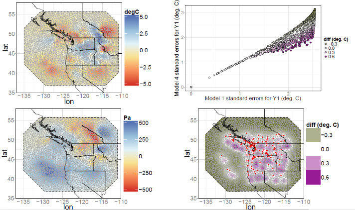
Figure 2: Left panels: The cokriged surface using maximum likelihood parameter estimates with an asymmetric model constructed using the conditional approach, for the temperature and pressure error fields. Top-right panel: A scatter plot of the kriging standard errors of $Y_1$ (temperature) obtained with the asymmetric model against those obtained when assuming $Y_1$ and $Y_2$ are two independent Matérn fields (the independent Matérn model), at each of the mesh vertices. The colour illustrates the difference between the two, with green denoting the higher standard error of the asymmetric model and purple the higher standard error of the independent Matérn model. Bottom-right panel: A spatial plot of the difference in the kriging standard errors of $Y_1$ (temperature) obtained with the asymmetric model and the independent Matérn model, with green denoting a higher standard error of the asymmetric model and purple a higher standard error of the independent Matérn model. The red dots denote the station locations.

Reproducible code

The code used in this work, that has been packaged and versioned, can be found here.

Apanasovich, T. V. and Genton, M. G. (2010). Cross-covariance functions for multivariate random fields based on latent dimensions. Biometrika 97, 15–30.

Banerjee, S., Carlin, B. P. and Gelfand, A. E. (2015). Hierarchical Modeling and Analysis for Spatial Data, 2nd edn. Boca Raton, FL: Chapman and Hall/CRC.

Cressie, N., and Zammit-Mangion, A. (2016). Multivariate spatial covariance models: A conditional approach. Biometrika, 103, pp. 915–935.

Gneiting, T., Kleiber, W. and Schlather, M. (2010). Matérn cross-covariance functions for multivariate random fields. Journal of the American Statistical Association 105, 1167–1177.

Schlather, M., Malinowrki, A., Menck, P. J., Oesting, M. & Strokorb, K. (2015). Analysis, simulation and prediction of multivariate random fields with package randomfields. Journal of Statistical Software 63, 1–25.

Authored by N. Cressie and A. Zammit-Mangion, 2015; revised 2020.