Local flux inversion

Bayesian Atmospheric tomography for detection and quantification of local-scale methane emissions

Detection and quantification of greenhouse-gas emissions is important for both compliance and environment conservation. However, despite several decades of active research, it remains predominantly an open problem. In 2015, a controlled-release experiment headed by Geoscience Australia was carried out at the Ginninderra Controlled Release Facility, and a variety of instruments and methods were employed for quantifying the release rates of methane and carbon dioxide from a point source.

The methodology presented below is ideally suited to quantifying local-scale leaks from industrial facilities or from the subsurface (e.g., well heads, buried pipelines or gas leakage up geological fractures and faults) where a surface leak has been detected but needs to be quantified. It can be used where physical access to the source location is limited, e.g., gas bubbling from a creek or where measurement is hazardous. Depending on the circumstance, detection of leakage can take many different forms, from visible bubble detection, optical gas imaging, handheld sniffers, noise detection, helicopters equipped with lasers, drones equipped with gas sensors, to monitoring die-off in vegetation using remote sensing techniques. Surface leakage typically expresses as small, concentrated hotspots if sourced from the subsurface (Feitz et al., 2014; Forde et al, 2019), for which the quantification approach outlined below is ideal. Equipment placement can be optimised around the leakage site (i.e., prevailing upwind/downwind) for optimal quantification.

Atmospheric tomography, a term inspired from medical imaging, combines data from a collection of measurement sites with Bayesian inversion to detect and quantify emissions. Inference in such cases is often done using Markov chain Monte Carlo (MCMC) sampling, because it allows relatively easy computation of posterior distributions of parameters that are deeply nested within a hierarchical model. It is also ideally suited for the case of point-source emissions, where the dimensionality of the latent space is low (unlike, for example, when doing regional emission quantification). The technique we describe is applicable to both point and path-sampling instruments, and accounts for uncertainty in the data, in the process models, and in the parameters.

Work presented on this page is joint between CEI and Andrew Feitz, Sangeeta Bhatia, Ivan Schroder, Frances Phillips, Trevor Coates, Karita Negandhi, Travis Naylor, Martin Kennedy, Steve Zegelin, Nick Wokker, and Nicholas M. Deutscher.

A full description of the experimental setup, measurement techniques and quantification methods used in the 2015 Ginninderra release experiment are given in Feitz et al. (2018). Briefly, CH$_4$ (together with CO$_2$ and nitrous oxide), was released from a small chamber located in a fallow agricultural field from 23 April to 12 June 2015, and 23 to 24 June 2015. A variety of CH$_4$ sensors were placed around the release chamber. The measurement data considered in this study were obtained from two Picarro analysers (labelled Picarro.West and Picarro.East, respectively), four eddy covariance (EC) towers equipped with open path CH$_4$ sensors (labelled EC.A, EC.C, EC.D, and EC.E, respectively), two scanning FTIR analysers with four retro-reflectors terminating six measurement paths (labelled P1 to P6, respectively), and a scanning Boreal laser with seven reflectors forming seven measurement paths (labelled R1 to R7, respectively); see Figure 1.

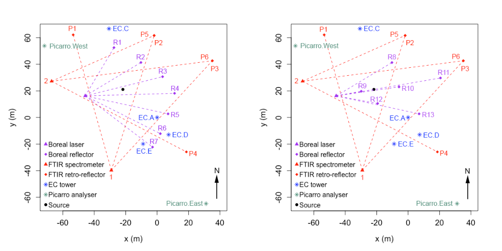
Figure 1. Left: Layout of instruments in the 2015 Ginninderra release experiment between 21 May and 7 June 2015. Right: Layout of instruments between 8 and 12 June 2015. R1 to R13 are the paths formed between the Boreal laser and reflectors; P1 to P6 are the paths formed between the FTIR spectrometers and retro-reflectors; EC.A to EC.E are the EC towers; and Picarro.East and Picarro.West are the Picarro analysers. All coordinates are relative to EC.A, which is situated at the origin.

CH$_4$ was released at a height of 0.3 m, at a standard release rate of 5.8 g min$^{-1}$, limited mostly to daylight hours. Towards the end of the experiment (8 to 12 June), the CH$_4$ release rate was decreased from 5.8 to 5.0 g min$^{-1}$ and the setup for the Boreal laser measurements was modified with the number of retro-reflectors and paths reduced to six (labelled R8 to R13, respectively; see the right panel of Figure 1). The Picarro analysers were not deployed until 21 May, and the CH$_4$ release rate on 23 and 24 June was constantly varied. Hence, here we only consider data between 21 May and 12 June, excluding 26 and 27 May where the release rate was also constantly varied. Measured CH$_4$ concentrations were then matched with corresponding meteorological measurements, on a common resolution of five minutes.

We model the CH$_4$ dispersion after release via a transport model that is simply parameterised, and easy to evaluate, so that it can be calibrated during the MCMC sampling. One of the simplest models that works well on the short distances we consider is the Gaussian plume dispersion model (e.g., Wark et al., 1998, Chapter 4). Denote the true emission rate by $Q$ in g s$^{-1}$, and the height of the CH$_4$ point source by $H$ in m. The classic Gaussian plume model is given by

$\begin{equation*} C(x_i, y_i, z_i, Q) = \frac{Q}{2\pi U_i \sigma_{y} \sigma_{z}} \exp\left(-\frac{y_i^2}{2 \sigma_{y}^2}\right) \left[\exp\left(- \frac{(z_i - H)^2}{2\sigma_{z}^2}\right) + \exp\left(-\frac{(z_i + H)^2}{2\sigma_{z}^2} \right)\right] \end{equation*}$

where $C$ is the model-predicted concentration in g m$^{-3}$ of CH$_4$ at a single spatial point $(x_i, y_i, z_i)$ in m along the direction of the plume corresponding to the $i$th measurement; $U_i$ is the wind speed associated with the $i$th measurement in m s$^{-1}$; and $\sigma_y, \sigma_z$ are the standard deviations in the horizontal and vertical directions, respectively. Figure 2 shows a horizontal cross section of the Gaussian plume dispersion model at a height of 1.5 m, and with concentrations in parts per million (ppm).

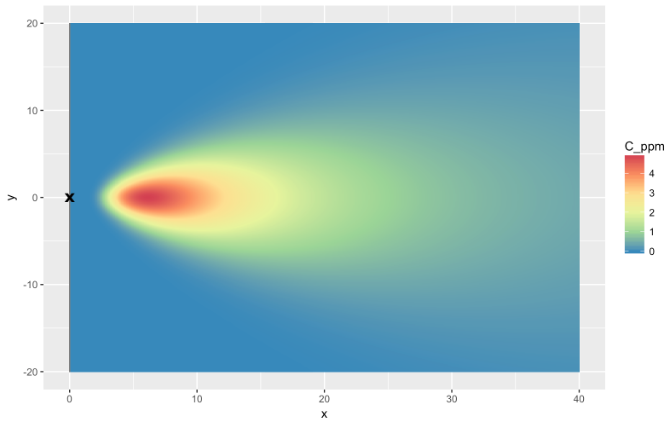
Figure 2. Horizontal cross section of the Gaussian plume dispersion model where $z_i =$ 1.5 m. Concentrations are in ppm.

We are ultimately interested in obtaining a range of plausible values for $Q$, a posteriori, (i.e., after we have collected the data). In this section we present a hierarchical statistical model that relates $Q$ to the observed concentrations via an atmospheric transport model (here, the Gaussian plume dispersion model).

Let $\boldsymbol{Y} \equiv (Y_1, Y_2, \dots, Y_N)'$ denote $N$ observed CH$_4$ enhancements (background-corrected concentrations). We model each $Y_i,\ i \in 1, 2, \dots, N$, as

$Y_i = C_i + \varepsilon_i,$

where $C_i$ is the $i$th atmospheric-transport-model-predicted CH$_4$ concentration, and $\varepsilon_i$ is the $i$th random error term, assumed to be Gaussian. The posterior distribution of the release rate $Q$ is then given by

$\begin{align*} p(Q \mid \boldsymbol{Y}, \boldsymbol{\Theta}) & \propto \int p(\boldsymbol{Y}, \boldsymbol{\Phi} \mid Q, \boldsymbol{\Theta})p(Q)\ \text{d}\boldsymbol{\Phi} \\ & = p(Q) \int p(\boldsymbol{Y} \mid Q, \boldsymbol{\Phi}, \boldsymbol{\Theta}) p(\boldsymbol{\Phi})\, \text{d}\boldsymbol{\Phi},\\ \label{bayes} \end{align*}$

where $\boldsymbol{\Phi}$ are model parameters, predominantly related to the Gaussian plume model, that we want to make inference on, $\boldsymbol{\Theta}$ are the model parameters that we assume are known, $p(Q)$ is the prior density of $Q$, and $p(\boldsymbol{Y} \mid Q, \boldsymbol{\Phi}, \boldsymbol{\Theta})$ is the Gaussian likelihood function.

Computation of the the posterior distribution $p(Q \mid \boldsymbol{Y}, \boldsymbol{\Theta})$ involves a high-dimensional integral that is analytically intractable. We therefore use MCMC, specifically a Gibbs sampler, to obtain samples from the posterior distributions of $Q$, and any other parameters on which inference is done. The Gibbs sampler samples each parameter one at a time from their respective full conditional distributions, where conditioning is done using the most recent samples of all other parameters. Generally, the prior distributions on these parameters are not conjugate priors, and hence the full conditional distributions for each of these are not available in closed form. We therefore use standard Metropolis-within-Gibbs to sample from these conditional distributions, with Gaussian proposals and adaptive scaling during the early stages of the MCMC algorithm.

The left panel of Figure 3 summarises our MCMC results for $Q$, using the real Ginninderra observations, and when the source was switched on. Full results are given in the first ten rows of Table A1 in Cartwright et al. (2019). While our posterior inferences are reflective of the true underlying emission rate, we see that with the real data the true values were not always captured within our 95% posterior credible intervals. This suggests that there are other important factors at play (e.g., with the meteorological data such as ambient temperature or wind direction, that we assume are fixed and known) that are not (or not fully) accounted for in our model. A close inspection of the residuals at EC.A revealed mild deviations from our Gaussianity assumption, while posterior predictive distributions on left-out EC tower data in a re-analysis revealed coverage probabilities that are slightly too large. Nevertheless, our worst-case scenario, obtained with the combination of all instruments in the 5.0 g min$^{-1}$ release-rate period, had an interval limit which was only 0.55 g min$^{-1}$ (approximately 11%) off from the true value, while all posterior medians were within 36% of the true value (within 22% if one ignored results from the Picarro analysers during the 5.0 g min$^{-1}$ release-rate period). This is encouraging because a single, common inference method was used to obtain the inferences from data at a common temporal resolution – no manual instrument-specific tuning was carried out. The approach thus seems relatively robust to instrument type.

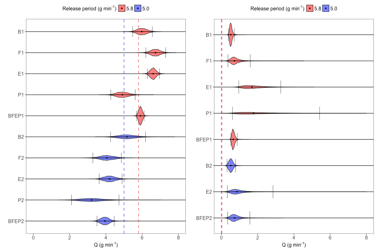
Figure 3. Left: posterior empirical distributions of the emission rate $Q$ in g min$^{-1}$, for the Boreals (B), FTIRs (F), EC towers (E), Picarro analysers (P), and the ensemble of all instruments (BFEP), for each release-rate period (1 and 2) during the Ginninderra experiment. The 5.8 g min$^{-1}$ release-rate period is shown in red (B1, F1, E1, P1, and BFEP1), while the 5.0 g min$^{-1}$ release-rate period is shown in blue (B2, F2, E2, P2, and BFEP2). The vertical dashed lines denote the respective true emission rates, the black dots denote the median estimates, and the black vertical bars denote the upper and lower limits of the 95% posterior credible intervals. Right: same as the left panel but showing results obtained using measurements taken when the methane point source was inactive. We can recover a reasonable range of estimates for the emission rate, with no 95% posterior credible interval being far from the true emission rate. Further, we see that the posterior emission rate credible intervals move towards zero when the source is inactive, as desired.

The right panel of Figure 3 summarises our results for $Q$ when the source is switched off, while full results are given in the second set of ten rows in Table A1 in Cartwright et al. (2019). Due to the choice of prior over $Q$ (a half-normal distribution), it is not possible for the 95% credible interval to include zero. Clearly, however, the intervals for $Q$ are close to zero and are suggestive of a small emission rate. As expected, the uncertainty is not well-constrained in this setting when the source is off: Narrow credible intervals on the emission rate here are only possible when the measurement is largely insensitive to the shape of the Gaussian plume. This is indeed the case for the Boreal paths, some of which pass very close to the source. With other instrument configurations, uncertainty in the plume scalings dominates. In some cases (FTIRs and Picarro analysers in the 5.0 g min$^{-1}$ release-rate period) our MCMC algorithm did not converge after 60000 samples (the chosen number of samples to take in each case); these results are thus omitted from Figure 3.

The work outlined here is described in further detail in the manuscript published in Atmospheric Measurement Techniques, available here.

The data and scripts required to reproduce the results in this article are available here.

Authored by L. Cartwright and A. Zammit-Mangion, 2020.