Scope

Slope Stability within Urban Areas, including along roads and railway lines

The importance of slope stability in the urban context must be highlighted in view of the increasing frequency of losses from landslides worldwide. The causes, triggering factors and mechanisms of occurrence are, of course, important. The traditional geotechnical approach involving investigation, testing, analysis, design and monitoring is still valid but is no longer sufficiently comprehensive in the urban context. Major aspects of landslide hazard must be considered including the expected volumes and magnitudes. The velocity and travel distance of a landslide can be critical factors on the capacity for damage or destruction Moreover, there should be an increasing focus on the elements at risk and on assessing the vulnerabilities of different areas and regions. Research is required to determine if regional or local vulnerabilities are increasing and for finding out the causes. A modern strategy for assessing regional landslide susceptibility and risk must include, among other things, the development of a landslide inventory, the preparation of GIS-based maps of existing landslides, the mapping of elements at risk and the collection and analysis of data on rainfall duration and intensity. Assessing uncertainties is important and the application of probabilistic approaches must be considered. An observational approach based on field monitoring of movements (surface and subsurface) and pore water pressures can prove to be very useful during research as well as during remediation of landslides.

Landslide movements which may be considered quite small and harmless in rural areas with very low population density cannot be neglected in a developed or developing urban area. There are many examples of damaging landslide movements with velocity classified as very slow In the Illawarra region of New South Wales, there are many examples of significant damage to residential houses, roads, railway lines and other infrastructure, all caused by landslides which move intermittently and slowly, the so-called stick-slip type of movement.

University of Wollongong GIS-based Landslide Inventory of the Wollongong region

The GIS-based Landslide Inventory comprises digital landslide datasets (shapefiles in an ESRI ArcGIS Personal Geodatabase), from which maps are generated of all the known landslide sites. The Landslide Inventory has existed now for over 10 years and has substantially grown in capacity every year since it was first developed (Chowdhury and Flentje 1998, Flentje and Chowdhury 2005). The Inventory currently includes almost 600 landslide sites with a total of almost 1000 landslide 'events' (including all known occurrences and recurrences). For example, Site 113 in Thirroul has 16 recurrences documented following its first recorded movement in March-April 1950.

The key identifier for each record in the Landslide Inventory is the Site Reference Code, being a decimal number with one significant figure, is unique for each landslide site. An abbreviated data dictionary for the 21 standard fields required for each landslide site is shown in Table 1 and the database record 'form' showing these standard fields is shown in Figure 2. The database has a total of 75 fields available for each site and a comprehensive data dictionary is included at the end of this document.

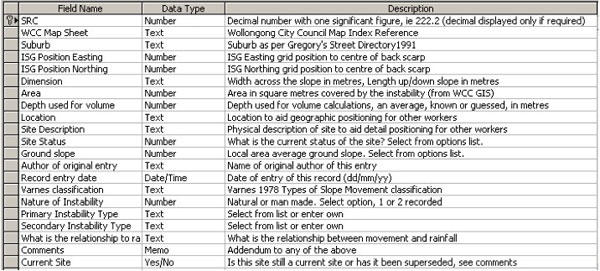
Table 1. Standard fields 'data dictionary' of the Landslide Inventory

One aspect of the Landslide Inventory that has been extremely useful is the listing per site of the first occurrence and any subsequent recurrences of each landslide site (Flentje and Chowdhury, 2002). Such a listing for Site 113 is shown in Figure 3. This information is important for the assessment of landslide frequency, and provides significant evidence of landslide hazard. For example Site 113 was first reported in April to March 1950, and was most recently active in October 2004, a period spanning 54 years. With the 17 landslide events known at this site, the average annual frequency of landsliding is 0.315. With additional information regarding magnitudes or rates of displacement at each event, the frequency of landsliding can be defined even more precisely. Such calculations can directly be used in the quantitative assessment of risk.

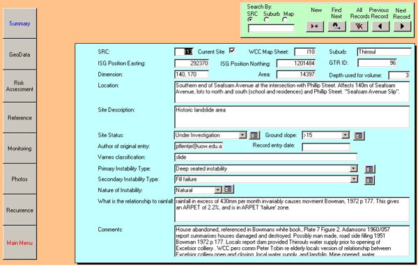
Figure 2. Database Record form showing the 22 standard fields for landslide Site 113.

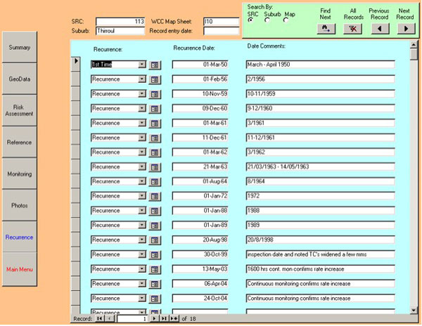
Figure 3. Landslide occurrence/recurrence data from Landslide Inventory for Site 113

In addition to the tabulated database, GIS-based maps of the known landslide locations can be prepared. An example of the mapping capability of GIS software is shown in Figure 4. GIS maps can be prepared at different scales, governed only by the resolution of the data displayed on the maps. One wall of the first writer's office is covered with 1:10,000 scale maps of the Wollongong region containing, as a background, a 10m Digital Elevation Model of the region, cadastre, geology and superimposed on this landslides colour coded by landslide type.

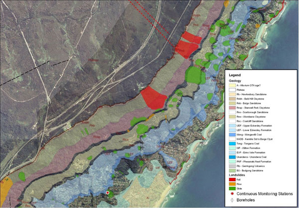
Figure 4. GIS-based map segment of the Scarborough and Wombarra areas in the northern suburbs of Wollongong. The geology of the escarpment area is shown as are the landslide areas.

The University of Wollongong Landslide Inventory is now well known in the New South Wales geotechnical community. It is increasingly being used as a reference source for a range of infrastructure developments being considered or already in progress in Wollongong. The following list summarises the projects that have sought regional and or site-specific landslide data from the Landslide Inventory to date:

• The Wollongong City Council and University of Wollongong landslide databases are combined to form one comprehensive Inventory
• Roads and Traffic Authority of New South Wales Alliance partnership review of Slope Hazards affecting the Lawrence Hargrave Drive between Clifton-Coalcliff. This was part of the process for the $54 million bridge construction project which is now in progress
• Rail Corporation of New South Wales review of landslide-triggering rainfall thresholds for the South Coast railway line
• The New South Wales Department of Urban Affairs and Planning Commission of Inquiry into the long term planning and management of the Illawarra Escarpment and its foothills
• Development of the Illawarra Escarpment Management Plan by the Wollongong City Council
• National Parks and Wildlife Service of New South Wales exposure to landslide risk along the Wollongong escarpment undertaken by URS Pty Ltd
• Assessment of the viability of a Rail Corporation of New South Wales realignment of South Coast railway line by Coffey Geosciences
• Sydney Water Corporation development of Low Pressure Sewerage Scheme for the four Wollongong northern towns of Otford, Stanwell Park, Stanwell Tops and Coalcliff
• University of Wollongong Landslide Research Team development of GIS-based landslide hazard maps for the WCC LGA using 'data mining' techniques.
• Daily operations of the WCC related to geotechnical management of landslides within the LGA.
• A variety of local and Sydney based geotechnical consultants daily operations related to management of landslides within the LGA and surrounding areas.
• Input of all Wollongong landslide locations into the Australian Landslide database managed by Geoscience Australia. 

This list of projects clearly demonstrates the importance of the valuable information the Landslide Inventory contains. Having the information in one accessible location adds value to every project that accesses the information. The alternative of not having the accurate information accessible, regularly updated and in such a flexible format is unthinkable in the difficult and challenging Wollongong terrain.

DATA DICTIONARY FOR THE LANDSLIDE DATABASE

Site Reference Code: Each of the sites of instability has been assigned a five character numeric Site Reference Code, or SRC, (included is one decimal point and one decimal place).

Wollongong City Council Map Index: Unique reference numbers are given to each individual 1:4000 map sheet by the WCC. A map index reference sheet is included in Chapter 1 as Figure 1.6. The WCC 1:4000 map sheet divisions are the same as the Australian Central Mapping Authority (CMA) 1:4000 map sheet divisions. Hence WCC map sheets correspond, for example, to the CMA ortho-photographic sheet, and cadastral, map boundaries. Table 1.1 displays the corresponding map sheet names for the WCC and the CMA. In the writers experience, the CMA 1:4000 ortho-photographic sheet maps are commonly used in the Illawarra (and elsewhere in NSW) for desktop geotechnical work. If a site crosses map sheet boundaries, all map sheets affected have been entered, separated by a comma, with no spaces.

Suburb: The suburb in which the site is located. The WCC official suburb boundaries have only recently been finalized. The suburb location of each site in the database has been determined on the basis of these finalized boundaries and is based on the location of the center of each landslide area.

ISG Grid Position Easting: Integrated Survey Grid (ISG) Easting of the approximate centre of the rear main scarp. ISG is one of several internationally recognised survey coordinate position reporting methods. All locations within subject area lie within ISG Zone 56-1. The WCC GIS package does, however, allow input and output using alternative coordinate systems (ie latitude and longitude).

ISG Grid Position Northing: Integrated Survey Grid (ISG) Northing of the approximate centre of the rear main scarp,

Dimension: Maximum width across the slope, and length up/down the slope, in metres.

Area: In square metres of the site. Value output from the WCC GIS and is based on the digitised area of the site,

Depth used for volume calculations: A known or estimated average depth to the actual or potential slip surface. Compare with Depth to Basal Shear.

Volume: In cubic metres of the site using a known or estimated average depth to the actual or potential slip surface multiplied by the area. Landslide volume is considered here to be a direct measure of the landslide magnitude.

Rank of Volume: A ranking from 1 to 319 of the volume, in decreasing size, of each landslide.

Location: Text description of geographic location of the site to aid positioning for other workers, for example; On the eastern side of George Street, opposite the council depot.

Site Description: Physical description of the site to aid perception and to assist detail positioning of site for other workers. The physical description is based on the judgement of the writer considering the contours shown on the 1:4000 topographic plans, and hence should be considered to be qualitative only,

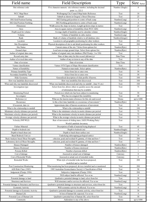
Table 5.1. Field descriptions, Field type and Size in Land Instability Database Table entitled 'SITES OF INSTABILITY'.

Site Status: Current site status regarding known land instability. Select from list of four options;

The number corresponding to the item selected, rather than the item itself, appears in the table SITES OF INSTABILITY. 

Ground slope: Local area ground slope. Select from list of three options;

The number corresponding to the item selected, rather than the item itself, appears in SITES OF INSTABILITY. The ground slope is based on the contours shown on the 1:4000 plans, and hence should be considered approximate. There are often local variations in slope inclinations within the general area. 

Author of original data entry: Author of original records data entry. For sites 1 to 328 the writer will be the author, Phil Flentje.

Record entry date: Original date of entry for this record. Default value of current date entered by computer for new sites when record opened for first time. All original dates will be between February 1996 and July 1997, the period during which the database was compiled and extensively validated.

Author of revised data entry: Author of any revision to any of the data within the record. Additional fields may be required if multiple revisions are required.

Date of revision: Date of any revision carried out. Revision dates can be entered manually in the format dd/mm/yy.

Varnes classification: Follows the classification system outlined by Varnes (1978) in his Figure 2.1, entitled 'Types of slope movement'. This classification system is outlined briefly in chapter 2 and table 2.1. Cruden and Varnes (1996) proposed a revision of this classification system as described in chapter 2, but Varnes' 1978 system has been adopted in this thesis as it is already widely accepted.

Nature of Instability: Identifies whether instability at the site is of natural or of man made origin. Select options from list;

The number corresponding to the item selected, rather than the item itself, appears in table SITES OF INSTABILITY. 

Primary Instability Type: A list of locally applicable general situations. This data field allows assessment of types of instability, overall review, and classification of different types of instability hazard. Select options from list;

Secondary Instability Type: Select options from list of situations, the same as in Primary Instability above. The secondary list reflects the fact that it is often difficult to distinguish a single factor responsible for the instability.

Slide Geometry: A generalised description of the shape of the profile of the shear surface(s), if known, or assumed.

How was the landslide discovered: How was the instability first discovered?

When and why was landslide discovered: When and why was the instability first discovered ? (ie, after June 91 rains).

Investigation type: Allows ready assessment of the amount of information that may be available (elsewhere) for a site. Select option from list;

Monitoring Period: Period over which site has been subject to monitoring (piezometers, inclinometers, survey, ...,etc)

Investigator: Name of individual(s) or company(s) that has investigated this site.

Reference (s): What was the source of the data. Name of author, company, date and report number(s), etc. Comprehensive reference list of these database cited references comprises separate table, REFERENCES, within the database file LI.MDB. A query lists these references alphabetically.

Recurrence: Is it a first time movement or a recurrence of an older event. Select option from a list;

The number corresponding to the item selected, rather than the item itself, appears in the table SITES OF INSTABILITY. 

If recurrent, date (s): Approximate date of known occurrences of movement. Whilst exact dates of movement are desirable (i.e, dd/mm/yyyy), month and year or year only have been entered if that is the best information available.

vWhat is the relationship to rainfall: Numerous workers in the past have examined the relationship of movement to rainfall at some sites. This may cover the response of one site in one time period, its history of movement, or it may be more general information. During this research project various antecedent rainfall periods have been considered; 7 days, 30 days, 60 days, 90 days and 120 days, termed herein as A7, A30, A60, A90 and A120 respectively. The relationship between these periods, their respective rainfall magnitudes and corresponding rates of movement (mm movement per period) are discussed in Chapters 8 and 9 in the PhD of Flentje. In addition, Antecedent Rainfall Percentage Exceedance with Time (ARPET) curves have been prepared as is discussed in Chapters 8 and 9. ARPET values (exceedance probabilities and antecedent rainfall magnitudes for specified antecedent periods, i.e, A7 or A90) are reported for some sites. A report of a query of the table SITES OF INSTABILITY, including site reference code, volume rank, map sheet, recurrence, WP/WLI velocity field (see below), the three velocity fields and this field 'What is the relationship to rainfall' is shown in Chapter 8, Table 8.2.

Minimum velocity (distance travelled per time period): Minimum velocity of landslide movement in metres per time period. Commonly determined by survey of pegs or monuments (movement of ground surface) or by inclinometer deflection (movement of shear surface at depth). Source of data, date and appropriate depth if available.

Maximum velocity (distance per period): Maximum velocity of landslide movement in metres per time period.

Average velocity (distance per period): Average velocity of landslide movement in metres per time period.

Velocity (WP/WLI): Estimated or reported maximum classified rate of movement of sliding mass. Classification used is that of the International Association of Engineering Geologists Working Party on the World Landslide Inventory (WP/WLI), which is based on the scale proposed by Varnes (1978). Select class from list displayed in table 2.3.

Failure Material: Very brief description of the bulk of the failure material.

Depth to bedrock (m): Average depth to bedrock in metres based on evidence or judgement.

Depth to basal shear (m): Depth to shear surface in metres based on evidence or judgement.

Basal Bedrock Unit (s): Geological bedrock units underlying the shear failure surface. Abbreviations used as per Bowman (1972) and summarised in Chapter 3 (see table here).

Back Analysis derived Shear Strength parameters: Cohesion, c (peak and residual), angle of internal friction, ∅ (peak and residual, and effective strength values), unit weight ϒ, of what type of material and how these values were determined.

Laboratory based Shear Strength parameters: Cohesion, c (peak and residual), angle of internal friction, ∅ (peak and residual, and effective strength values), unit weight ϒ, of what type of material and how these values were determined.

Houses Damaged: Number of houses damaged.

Houses Destroyed: Number of houses destroyed.

Persons Killed: Number of persons killed.

Cost of damage: Assessed or actual cost of damage.

Cost of Remedial Works: Assessed or actual cost of remedial works.

Remedial Works: What style of remedial works has been proposed, modelled and or installed, and when. Type and number of subsurface drains, length and number of piers, dewatering wells,..., etc.

Post Construction Monitoring: What types of monitoring systems have been proposed, devices installed to monitor performance since installation of remedial works? What do the results of any monitoring suggest about the current status of the site?

AGS Risk Classification (1985): Australian Geomechanics Society, Classification of Risk of Instability (1985) Risk Classification. By AGS definition, all sites included in this database are classed as Very High Risk or High Risk. NOTE: a major challenge for the future is to be able to carry out more sophisticated and detailed hazard and risk assessments of each of these sites.

Judgement (Flentje 1996): Subjective judgement, by the writer, on the basis of available information. In some cases, this judgement was not possible, as the writer was not familiar with the site. Judgement regards current status of the landslide based on knowledge and experience.

The following items are also subjective judgements by the writer regarding the three elements inferred by Varnes (1984), namely structures and services, economic activity and human life, plus one additional element, land. Qualitative element vulnerability is also presented.

strong>Land: Will the subject land be affected by the reasonably expected, or even exceptional, continued movement associated with the instability. Binary yes or no, -1 or 0, respectively. The number corresponding to the item selected, rather than the item itself, appears in the table SITES OF INSTABILITY.

Potential damage to land: Potential for damage to land, select option from following list:

Future research in consultation with local government and other authorities and experts is needed to establish quantitative definitions of each of these categories. 

Structures and Services: Is it likely that the structures and services are going to be affected by the reasonably expected or, even exceptional, continued movement associated with the instability. This item was also inferred by Varnes (1984). Binary yes or no, -1 or 0, respectively. The numbers corresponding to the item selected, rather than the item itself, appear in the table SITES OF INSTABILITY.

Potential damage to Structures and Services: Potential for damage to structures and services, select option from following list:

These above options have been adapted with two additions from the Australian Standard Residential Slabs and Footings (AS 2870.1). The two levels of damage which have been added here, by the writer are, 'no damage potential' and 'complete destruction'. 

Economic Activity: Is the economic activity related to the subject land likely to be affected by the reasonably expected or, even exceptional, continued movement associated with the instability. This item was also inferred by Varnes (1984). Binary yes or no, -1 or 0, respectively. The number corresponding to the item selected, rather than the item itself, appears in the table SITES OF INSTABILITY.

Potential damage to Economic Activity: Potential for damage to, or loss of, economic activity. Select option from following list:

Human Life: Is loss of human life likely under reasonably expected or, even exceptional, continued movement. This item was also inferred by Varnes (1984). Binary yes or no, -1 or 0, respectively. The number corresponding to the item selected, rather than the item itself, appears in the table SITES OF INSTABILITY.

Potential Loss of Human Life: Potential for loss of human life. Select option from following list:

This potential for loss of life as a consequence of landsliding relates to only one human life. It is beyond the scope of this thesis, to determine the exposure of the general population to the effects of the instability or failure of an individual site. It would be appropriate, however, for such exposure to be considered in more focused individual projects concerned with hazard and risk assessment. 

Comments: A field for memo type entries up to 255 characters as an addendum to any of the above fields.

Landslide Susceptibility and Hazard derived from a Landslide Inventory using Data Mining

The University of Wollongong landslide research team has developed a comprehensive GIS-based Landslide Inventory of the 550 km2 Wollongong Local Government Area (WLGA) and surrounding regions, just south of Sydney in the State of New South Wales, Australia. This inventory includes almost 600 landslide sites and forms the crucial centrepiece of the methodology reported herein. The landslide inventory is described in the previous section of this web facility under the heading  Wollongong Regional Landslide Inventory. The inventory identifies 2.95% of a 188 km² escarpment study area to be covered by landsliding reported during the last 120 years. The landslides within the inventory comprise 42 falls, 43 flows and 480 slides according to the Cruden and Varnes 1996 classification. In addition, there are several scour related sites and a few that have not been classified. A total of 426 slide category landslides are located within the 188 km² Model area.

With GIS-based data sets, a 'slide' category landslide susceptibility map layer has been developed with the aid of 'knowledge-based' data-mining techniques. Susceptibility zones have been classified as (a) known landslides, (b) high susceptibility with ∼ 8% of the area subject to landslides (contains 57% of the known landslides), (c) moderate susceptibility with 4% of the area subject to landslides (contains 35% of known landslides), (d) low susceptibility with 0.85% of the area subject to landslides (contains 3.7% of known landslides), and (e) very low susceptibility with <0.1% of the area subject to landsliding (represents 71% of the study area). It is important to note that the high susceptibility zone identifies over 2,300 hectares of land, outside of known landslides, as being highly susceptible to landsliding. The 'slide' category susceptibility maps have been upgraded to hazard level maps with identification and labelling of site specific frequency, volume and 'profile' angles for each landslide. The average landslide frequency of occurrence for each susceptibility zone has been determined.

ADDITIONAL DATA SETS

In addition to the GIS-based landslide inventory, other GIS-based data sets have been developed for this project including engineering geological mapping, data acquired through external agencies and data sets generated by the GIS software using the Digital Elevation Model. In total, ten GIS-based data sets have been compiled. The data sets include:

• Geology (21 variables representing the mapped geological formations)
• Vegetation (15 variables representing the mapped vegetation categories)
• Slope Inclination (continuous floating point distribution)
• Slope aspect (continuous floating point distribution)
• Terrain Units (buffered water courses, spur lines and other intermediate slopes)
• Curvature (continuous floating point distribution)
• Profile Curvature (continuous floating point distribution)
• Plan Curvature (continuous floating point distribution)
• Flow Accumulation (continuous integer)
• Wetness Index (continuous floating point distribution)  

GIS-BASED DATA PREPARATION FOR DATA MINING

GIS facilitates the overlaying of disparate data sets using the spatial properties of the data. While GIS is a great mapping tool, it also facilitates analyses that evaluate relationships between various spatial systems in order to quantify processes and phenomena. All the datasets have been assembled into one ESRI ArcMapTM document. With the aid of the GIS application extension Hawths Analysis Tools (Beyer, 2005) and the Intersect Point Tool it contains, an ASCII xyz output file was produced for the specific purpose of a Data Mining (DM) analysis using the See5 software. The ASCII xyz output file incorporates the fully attributed data from each of the 1.88 million pixels of the model, for each of the eleven input layers.

The GIS capabilities have been combined here with the power of the knowledge-based DM software See5. Heuristic 'data mining' is the science of computer modelling of a learning process. The DM learning process extracts patterns from large databases, whether they are concerned with organisational processes or, as in this case, natural phenomena. These patterns can be used to gain insight into aspects of the phenomena, and to predict outcomes (in this case, pixels with characteristics matching those of known landslides) as an aid to decision-making. The DM process used in this application is outlined in Figure 3.

Figure 3. Flow chart outlining GIS-based and Data Mining methodology used to develop Slide Category Landslide Susceptibility Zoning Maps for the Wollongong City Council Area.

The See5 software is a well developed commercial progression of the seminal work surrounding its predecessor, C4.5 (Quinlan, 1993). Both software products have been utilised in a diverse range of domains including, complex signal processing and control Stirling (2002), dynamic spatiotemporal contexts (Sun et. Al. 2006, Zulli and Stirling, 2005 and Stirling 2005), as well as numerous spatial contexts using GIS (Huang et al 2001, Xian, 2002).

Early work on this methodology, proposed by the University of Wollongong, was carried out in collaboration with Geoscience Australia (Chowdhury et al, 2002).

THE DATA MINING PROCESS

The DM approach uses a training subset of the full data set of 1.88 million pixels. The training subset includes all of the landslide xy points (29,480 points), and to balance the numerical output of the model, an approximately similar number (a whole number proportion of the remaining total non landslide points) of randomly selected non landslide xy points (35,815 points). Hence, the complete training subset (in this instance) totals 65,295 points (3.47%), each representative of the centre point of a 10m² pixel, of the total 1.88 million points.

The See 5 software examines the training data and develops a symbolic Decision Tree which defines the data. Each arm of the Decision Tree defines a Rule Set (Table 1). The See 5 software examines both aspects of the training data (the landslide and non-landslide components) and cross validates the set of rules developed independently for each component with the opposing set to determine rule confidence values. The confidence values vary from -1 to 1, the non landslide 'confidence' values varying from-1 to 0, whilst the landslide 'confidence' values vary from 0 to 1. The number of rules produced by the model can be pre-set by the user and this variable determines the precision of each rule. Clearly, with more rules, the conditions defined by each rule will become more and more specific.

DATA MINING RULES

The Model, containing a number (R) of contextually sensitive rules, essentially maintains a judgement committee of R multiple hypotheses. The rules generated for this model are shown in Table 1. Each rule is ranked with a confidence factor, after evaluation and validation, by the Laplace Ratio (n-m+1)/(n+2) where n is the number of training cases that a specific rule correctly recognises and m, if it appears, is the number of cases that do not belong to the class predicted by the rule (class 1 = landslide, class 0 = not landslide). In addition, a measure of the gain potential, or lift, of each rule is also assessed, which is the ratio of each ruleÍs confidence relative the frequency in the training set of its class prediction.

Table 1. Rule Set for Slide Category Landslide Susceptibility

Rule 1: (736/15, lift 1.8)

 Rule 2: (20309/488, lift 1.8)

Rule 3: (22, lift 1.7)

 Click here to view all rules; from Rule 1 to Rule 40

Default class: 0

Evaluation on training data (65212 cases):

When multiple rules respond in order to classify a pixel, an aggregation resolution of their individual decisions (class predictions) is formulated, using the weighted confidence of each rule. Rule sets are then applied to the Entire Model Area. For efficiency, the trained model (represented by the rule sets) is also maintained as a compiled binary object, which can be further utilised by other programs for comparative or predictive purposes. To this end, a specialised prediction program was written to process the complete data set of 1.88 million pixels.

For every candidate pixel, the ultimate susceptibility is judged to be the aggregation of all rule confidences (both positive or negative/slide or no slide) that apply, as more than one rule often applies to each pixel. Apart from this, all of the responding rules are also noted for further analysis. These predicted values and features are later merged with the pixel coordinates into an ASCII text file, which is in turn managed (read) by the GIS.

• List of all 40 rules

PERFORMANCE OF "KNOWLEDGE BASED" DATA MINING MODELLING

To aid in the post DM analyses of the modelled confidence distribution, a script was written in Visual Basic code. This code ranked the data according to decreasing model confidence and determined the cumulative percent of data each value represented in the ranked list. Figure 4 shows the distribution of DM model 'confidence' for the preferred final slide model. The graph displays two curves, the upper red curve shows the distribution of model confidence for the landslide pixels, and the green lower curve shows the distribution of model confidence for each pixel in the entire model (1.88 million points). The graph highlights the excellent performance of the modelling. This is highlighted with the high model confidence for a very high proportion of actual landslides (red curve). As expected, a smaller but significant proportion of the area as a whole (green curve) is also predicted with a relatively high confidence.

Figure 4. Distribution of model Confidence for both the landslide training points (red) and the entire model area (green) versus percent of data for the c5m75 model.

Also shown on Figure 4, is the selected data mining 'confidence' based Landslide Susceptibility zone boundaries as summarised in Table 2. The 'confidence' values used to define the Susceptibility zone boundaries are arbitrary values. A segment of the Landslide Susceptibility map is shown in Figure 5. However, the quantitative review process which is summarised here validates the process and ensures it is completely transparent and open for review. Field validation is also used as summarised in the following section.

As summarised in the abstract, the DM modelling of Landslide Susceptibility has derived significant groupings and allowed well defined zones as shown in Figures 4, 5 and Table 2. The mapped landslides have been shown as a Susceptibility class on there own. Other susceptibility zones have been classified as (a) high susceptibility with ∼ 8% of this area subject to landslides and containing 57% of the known landslide population, (b) moderate susceptibility with 4% of this area subject to landslides (contains 35% of known landslides), (d) low susceptibility with 0.85% of area subject to landslides (contains 3.7% of known landslides), and (e) very low susceptibility with <0.1% of the area subject to landsliding and yet representing 71% of the study area. The high susceptibility zone identifies over 2,300 hectares of land, outside of known landslides, as being highly susceptible to landsliding. Furthermore, the model also identifies over 13,000 hectares as having a very low susceptibility to landsliding.

Table 2. Susceptibility Classification showing % of Study Area coverage and % of Slide category landslides population per class

Figure 5. Segment of the Landslide Susceptibility Map. Legend as shown in Table 2. Underlying grid is 1km square and North is towards the top right diagonal of the figure. The inset shows the hazard labelling, as described below, for one landslide, Site 113.

SUMMARY

In summary, the susceptibility zones have been classified as (a) high susceptibility with 8.12% of this area subject to landslides and containing 60.3% of the known landslide population, (b) moderate susceptibility with 4.12% of this area subject to landslides (contains 32.3% of known landslides), (d) low susceptibility with 0.85% of area subject to landslides (contains 3.3% of known landslides), and (e) very low susceptibility with 0.09% of the area subject to landsliding (contains 4.1% of known landslides) and yet representing 70.9% of the study area. These statistics are compatible with Table 4 of AGS (2007a). The high landslide susceptibility zone identifies over 2,300 hectares of land, outside of known landslides, as being highly susceptible to landsliding. Furthermore, the model also identifies over 13,000 hectares as having a very low susceptibility to landsliding.