CORGI: Change Of Resolution in GLM Inference

Scientific studies often involve exploring a regression-type relationship between a response and a set of purported explanatory variables, which can then be used to inform decision-making. An example of such a relationship, which will be illustrated throughout this project, is modelling a biodiversity response (eco-process) to climate conditions (geo-data). Once this relationship is learned, it can be used to predict biodiversity as climate changes.

The GLM (Generalised Linear Model) is a powerful statistical model for this type of analysis, as it accommodates different types of data (e.g., count and binary outcomes). In a spatial context, valid inferences from a GLM follow when the spatial resolutions of response data and data on explanatory variables match. However, response data such as species diversity is usually at a finer spatial resolution than that of explanatory climate data. Figure 1 highlights an example: Soil temperature (explanatory variable) data are available at a much coarser resolution than moss presence-absence data (Gore et al., 2023) in the southern Bunger Hills. As an ice-free area, Bunger Hills is a small coastal region that is topographically complex with a large number of standing water ice bodies; see Figure 2 for a photo of Bunger Hills and its location in Antarctica. In fact,  the vast majority of known terrestrial biodiversity in Antarctica is restricted to ice-free areas, which occupy a small fraction of the entire landmass. As such, modelling of Antarctic biodiversity in response to environmental change typically requires environmental data at a resolution finer than currently available.

Figure 1: The sampling sites of moss presence-absence data (left panel) were specified at a much finer resolution than that of the available soil-temperature data (right panel) from the ERA5 climate renalysis product.

Figure 2: Left panel: The Bunger Hills and Denman Glacier are about 440km away from Australia's Casey research station (source: Australian Antarctic Division). Right panel:  A photo of the Bunger Hills during the summer (source: Bruce Wilson).

Recognising the change-of-resolution problem and solving it is critical for well-informed decision-marking about, for example, conservation priorities in the face of climate change (e.g. Jansen et al., 2022; Lu and Jetz, 2023). This project tackles the challenge of resolution mismatch and develops approaches for making reliable inferences from GLMs when spatial resolutions do not align. In an article published in Methods in Ecology and Evolution (Zheng et al. 2025), we introduce a two-stage protocol in which the coarse-resolution data on explanatory variables are first downscaled through Monte Carlo sampling, followed by incorporating the downscaled samples in GLM inference, as explained below. Since implementing the protocol involves a change of spatial resolution in explanatory variables, we call the implementation of the protocol, CORGI (Change Of Resolution in GLM Inference).

To address the problem of resolution mismatch, we first need to downscale data on explanatory variables to the resolution of the response data. This has been tackled in the first stage of the protocol, ‘Spatial-statistical downscaling’. Using the downscaling method illustrated there, we obtain Monte Carlo samples of explanatory variables at a common fine-scale resolution, which we refer to as the downscaled samples. Figure 3 shows the means and standard deviations of the downscaled soil-temperature samples in Southern Bunger Hills, calculated for each basic areal unit (BAU) at $1\times1\thinspace{\rm km}^2$ resolution obtained from coarse-resolution $(5\times11\thinspace{\rm km}^2)$ ERA5 reanalysis data.

Figure 3: Soil-temperature prediction (mean of the soil-temperature downscaled samples), with sites where moss was present (triangles) in background (left panel); and standard deviation of the soil-temperature downscaled samples (right panel).

Next, we incorporate these downscaled samples in GLM inference. At the core of our framework is a spatial Berkson-error model. Berkson error happens when data on explanatory variables are not obtained, collected, or measured imperfectly (Carroll et al., 2006). In this model, an explanatory variable at fine resolution, say $X^{\left(f\right)}\left(s_i\right)$ on the BAU located at $s_i$, is decomposed into two components:
$$X^{\left(f\right)}\left(s_i\right)={\hat{X}}^{\left(f\right)}\left(s_i\right)+\eta^{\left(f\right)}\left(s_i\right),$$
where ${\hat{X}}^{\left(f\right)}\left(s_i\right)$ is the mean of the downscaled samples at the $i$-th BAU, and $\eta^{\left(f\right)}\left(s_i\right)$ represents a downscaling error. Importantly, the downscaling error is spatially correlated, reflecting the natural spatial structure and heterogeneity of environmental processes.

Recall that a GLM with an explanatory variable can be written as, for $i=1, \dots, n\thinspace$,
$$\begin{aligned} \left[Z^{\left(f\right)}\left(s_i\right)\thinspace|\thinspace Y^{\left(f\right)}\left(s_i\right)\right] &=EF\left(Y^{\left(f\right)}\left(s_i\right)\right),\\ g\left(Y^{\left(f\right)}\left(s_i\right)\right) &=\beta_0+\beta_1X^{\left(f\right)}\left(s_i\right),\\ \end{aligned}$$
where $Z^{\left(f\right)}\left(s_i\right)$ is the response data; $\left[Z^{\left(f\right)}\left(s_i\right)\thinspace|\thinspace Y^{\left(f\right)}\left(s_i\right)\right]$ denotes the conditional distribution of $Z^{\left(f\right)}\left(s_i\right)$ given $Y^{\left(f\right)}\left(s_i\right)$; EF is a distribution that belongs to an exponential family such that $E\left(Z^{\left(f\right)}\left(s_i\right)\thinspace|\thinspace Y^{\left(f\right)}\left(s_i\right)\right)=Y^{\left(f\right)}\left(s_i\right)$; $g\left(\cdot\right)$ is a link function, with unknown parameters $\beta_0$ and $\beta_1$ and a single covariate $X^{\left(f\right)}\left(s_i\right)$. Of particular interest is $\beta_1$, the coefficient of the climate explanatory variable $X^{\left(f\right)}\left(s_i\right)$.

To account for the downscaling uncertainty properly, both components, ${\hat{X}}^{\left(f\right)}\left(s_i\right)$ and $\eta^{\left(f\right)}\left(s_i\right)$, are included in the GLM for inference, as follows:
$$\begin{aligned} g\left(Y^{\left(f\right)}\left(s_i\right)\right)&=\beta_0+\beta_1X^{\left(f\right)}\left(s_i\right)\\ &=\beta_0+\beta_1\left({\hat{X}}^{\left(f\right)}\left(s_i\right)+\eta^{\left(f\right)}\left(s_i\right)\right)\\ &=\beta_0+\beta_1{\hat{X}}^{\left(f\right)}\left(s_i\right)+\delta^{\left(f\right)}\left(s_i\right).\\&\\ \end{aligned}$$

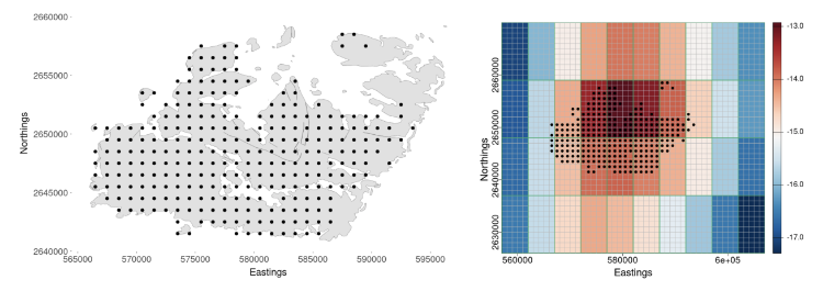
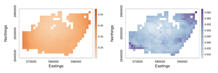
Here, the downscaling uncertainty is incorporated through the component $\delta^{\left(f\right)}\left(s_i\right)\equiv\beta_1\eta^{\left(f\right)}\left(s_i\right)$, which is seen to be the downscaling error $\eta^{\left(f\right)}\left(s_i\right)$ scaled by $\beta_1$. The simulation results in Figure 4 show why including the downscaling error matters: Inference using CORGI (colour blue) is valid compared to the commonly used ‘plug-in’ approach (colour green), which simply substitutes ${\hat{X}}^{\left(f\right)}\left(s_i\right)$ without accounting for the error (i.e., $g\left(Y^{\left(f\right)}\left(s_i\right)\right)=\beta_0+\beta_1{\hat{X}}^{\left(f\right)}\left(s_i\right)$). Another approach called ‘ensemble’ (colour red), shown in Figure 4 directly includes downscaled samples without using the Berkson-error decomposition (i.e., $g\left(Y^{\left(f\right)}\left(s_i\right)\right)=\beta_0+\beta_1{\widetilde{X}}^{\left(f\right)}\left(s_i\right)$, where ${\widetilde{X}}^{\left(f\right)}\left(s_i\right)$ is a downscaled sample). While the ‘ensemble’ approach seems intuitively appealing, it can lead to biased and invalid inferences. Recall that CORGI incorporates downscaling uncertainty in GLM inference. Figure 5 demonstrates Monte Carlo downscaled samples of $\mathbf{X}^{(f)} = (\mathit{X}^{(f)}_{(s_1)}, \dots, \mathit{X}^{(f)}_{(s_N)})^{\top}$ and Monte Carlo samples of $\mathbf{Y}^{(f)} = (\mathit{Y}^{(f)}_{(s_1)}, \dots, \mathit{Y}^{(f)}_{(s_N)})^{\top}$.

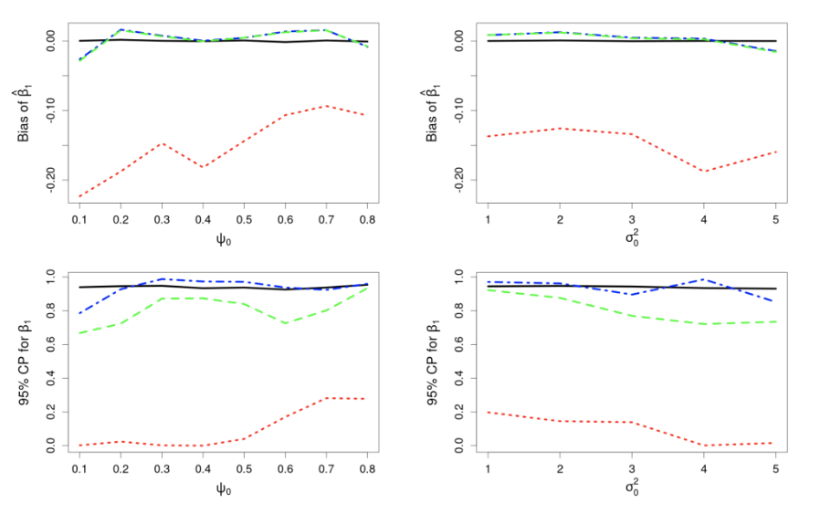
Figure 4: Comparison of CORGI (blue) to other methods, ‘plug-in’ (green) and ‘ensemble’ (red): Bias of estimate ${\hat{\beta}}_1$ against spatial range $\psi_0$ and spatial variance $\sigma_0^2$, respectively (top row); coverage probability (CP) for $\beta_1$ against spatial range $\psi_0$ and spatial variance $\sigma_0^2$, respectively (bottom row). The black line represents the ‘gold standard’ as a GLM was fitted with the ‘ground truth’.

Figure 5: (left panel) 100 Monte Carlo samples of $\mathbf{X}^{(f)}$; (right panel) 100 Monte Carlo samples of $\mathbf{Y}^{(f)}$ under CORGI.

So far, we have introduced the second stage of our (CORGI) protocol. Returning to the moss-data example in the southern Bunger Hills, Figure 3 shows the results from the first stage of our protocol, where we obtained the downscaled soil-temperature samples.

Figure 5 maps the mean and standard deviations of the moss-presence probability. These results correspond to the second stage of our protocol, where we fitted a Bernoulli GLM that incorporates the downscaled samples via the Berkson-error relationship. In particular, the model is given by

$$\begin{aligned} \left[Z^{\left(f\right)}\left(s_i\right)\thinspace|\thinspace Y^{\left(f\right)}\left(s_i\right)\right]&=Bernoulli\left(Y^{\left(f\right)}\left(s_i\right)\right),\\ g\left(Y^{\left(f\right)}\left(s_i\right)\right)&=\beta_0+\beta_1{\hat{X}}^{\left(f\right)}\left(s_i\right)+\delta^{\left(f\right)}\left(s_i\right),\\ \end{aligned}$$

where $Z^{\left(f\right)}\left(s_i\right)=1$ if mosses were present at site $s_i$, and $Z^{\left(f\right)}\left(s_i\right)=0$ otherwise; $Y^{\left(f\right)}\left(s_i\right)$ represents the moss-presence probability; and $g\left(y\right)=log\left(y/\left(1-y\right)\right)$ for $y\in\left(0,1\right)$ is a logit function. Our goal is to make inference on both $\beta_1$ and $Y^{\left(f\right)}\left(s_1\right),Y^{\left(f\right)}\left(s_2\right),\ldots$.

The result suggests that, on average, lower soil temperatures are associated with higher moss-presence probabilities in the southern Bunger Hills. Larger prediction uncertainties appear in pixels where mosses were not found or not surveyed and soil temperatures were relatively low. In addition, large soil-temperature downscaling uncertainties on individual pixels give larger moss-presence probabilistic uncertainties.

Figure 6: Mean (left panel) and standard deviation (right panel) of the predictive distribution of the moss-presence probability.

The work above was supported by Australian Research Council SRIEAS Grant SR200100005 Securing Antarctica’s Environmental Future (SAEF) funding and is described in the following article:

Zheng, X., Cressie, N., Clarke, D. A., McGeoch, M. A., and Zammit-Mangion, A. (2025). Spatial-statistical downscaling with uncertainty quantification in biodiversity modelling. Methods in Ecology and Evolution, 16, 837–853. https://doi.org/10.1111/2041-210X.14505.

All data and code are available at https://doi.org/10.5281/zenodo.14600559 (Zheng et al., 2025).

Carroll, R. J., Ruppert, D., Stefanski, L. A., & Crainiceanu, C. M. (2006). Measurement Error in Nonlinear Models: A Modern Perspective. Chapman and Hall/CRC. https://doi.org/10.1201/9781420010138.

Gore, D., Leishman, M., & Gibson, J. A. (2023). Biogeography of the Bunger Hills—plant and bird locations 1995-2000. Australian Antarctic Data Centre. https://doi.org/10.26179/563m-p165.

Jansen, J., Woolley, S. N., Dunstan, P. K., Foster, S. D., Hill, N. A., Haward, M., & Johnson, C. R. (2022). Stop ignoring map uncertainty in biodiversity science and conservation policy. Nature Ecology & Evolution, 6, 828–829. https://doi.org/10.1038/s41559-022-01778-z.

Lu, M., & Jetz, W. (2023). Scale-sensitivity in the measurement and interpretation of environmental niches. Trends in Ecology & Evolution, 38, 554–567. https://doi.org/10.1016/j.tree.2023.01.003.

Zheng, X., Cressie, N., Clarke, D. A., McGeoch, M. A., & Zammit-Mangion, A. (2025). Spatial-statistical downscaling with uncertainty quantification in biodiversity modelling using CORGI (Change Of Resolution in GLM Inference). Zenodo. v0.1.0. https://doi.org/10. 5281/zenodo.14600559.