Spatial-Statistical Downscaling

Regional or local analyses of bio-data (e.g., species diversity) often involve geo-data as explanatory variables (e.g., climate). Species-diversity data are typically at fine spatial scales, but in many circumstances, in situ measurements of climate data are either unavailable or sparse, because collecting them can be impractical or prohibitively expensive. Remote-sensing data (e.g., observations collected by satellites) provide useful alternatives, but such data sets can require specialised technical expertise to process and are usually available only at relatively coarse spatial resolutions, often coarser than species-diversity data.

Nevertheless, a common workflow in ecological studies, when fine-resolution climate data are not available, is to downscale coarse-resolution data given by numerical models, including general circulation models and climate reanalyses (e.g., ERA5; Hersbach et al., 2020). Downscaling explanatory variables from coarse resolution to fine resolution shows local details and spatial patterns that may not actually be present, and hence the downscaling comes with uncertainty. What is certain is that fine-resolution aggregates to the known coarse-resolution data. It is essential for drawing scientifically valid conclusions to quantify this uncertainty. Hence, we apply techniques from spatial statistics (Cressie, 1993; Ma et al., 2019; Zammit-Mangion et al., 2015) to statistically downscale data and provide valid uncertainty quantification, which represents the first stage of a two-stage protocol for inference on fine-scale eco-processes from coarse-scale geo-data.

Figure 1 illustrates various data sources commonly used for downscaling, and Figure 2 demonstrates the statistical challenges in downscaling coarse-resolution data. Figure 3 presents a real-world example, where moss data were collected at a fine ($1\times1\thinspace{\rm km}^2$) resolution from two expeditions to Bunger Hills in East Antarctica (Gore et al., 2023). In order to predict moss presence using climate, data from the coarser resolution (approximately $5\times11\thinspace{\rm km}^2$) ERA5 climate reanalysis product are used. Then statistical downscaling follows.

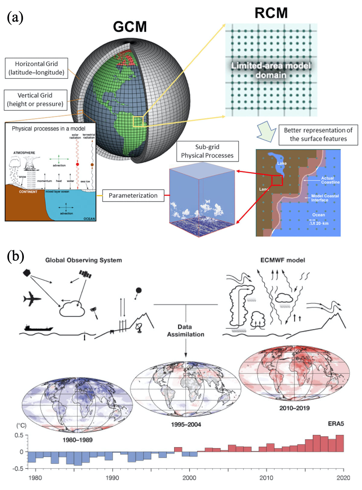
Figure 1: Data sources commonly used for downscaling: (a) A General Circulation Model (GCM) providing boundary conditions for an RCM (Regional Climate Model) (Image credit: Ambrizzi et al. (2019)); (b) A reanalysis climate product that uses assimilation and numerical models (e.g., ECMWF) together, for example, the ERA5 renalysis data (Image credit: ECMWF). In each case, their resolutions are usually too coarse for species-diversity studies.

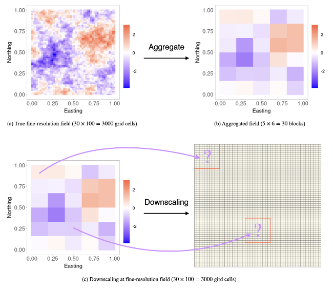
Figure 2: (a) A true fine-resolution field, which is aggregated; (b) The coarse-resolution aggregated field; (c) Downscaling to recover (a) from (b).

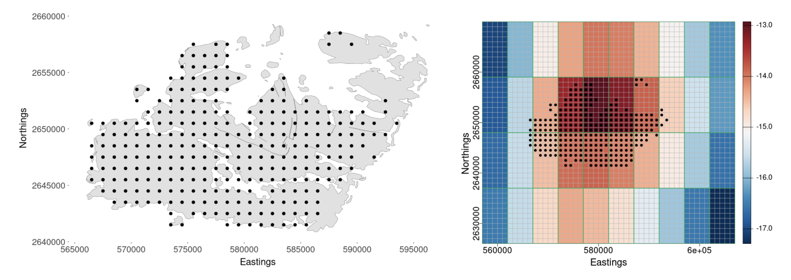
Figure 3: (a) Moss-data sampling sites in Southern Bunger Hills (fine resolution); (b) ERA5 soil-temperature data (coarse resolution) with the sampling sites in the background.

Our spatial-statistical downscaling framework involves three main steps:

Step 1: Specify a statistical model for the fine-resolution climate field using knowledge about the physics at fine resolutions.

Step 2: The parameters in the model from (i) are present in aggregations of the model. Estimate the parameters from the coarse-resolution climate data using the appropriately aggregated statistical model.

Step 3: Use the estimated parameters from (ii) in a conditional probability model (conditional on the coarse-resolution data) to generate samples of the fine-resolution field via conditional simulations.

Step 1: Specify a fine-resolution field

We represent the fine-resolution climate field as $\mathbf{X}^{(\mathit{f})}\thinspace=\thinspace\left(\mathit{X}\left(\mathit{s_1}\right), \dots, \mathit{X}\left(\mathit{s_N}\right)\right)^{\top}$ where each $\mathit{s_1},\thinspace\dots,\thinspace\mathit{s_N}$ represents a basic areal unit (BAU; Nguyen et al., 2012). The size of the BAU corresponds to the desired resolution from scientific consideration. We assume that this climate field $\mathbf{X}^{(\mathit{f})}$ follows a multivariate Gaussian distribution derived from a Gaussian process with unknown parameters $\mathbf{θ}$ in both the mean function and the spatial covariance function. We call this a GPB (Gaussian Process over BAUs). The distribution of $\mathbf{X}^{(\mathit{f})}$ given the parameters $\mathbf{θ}$ is denoted as [$\mathbf{X}^{(\mathit{f})}\thinspace|\thinspace\mathbf{θ}$].

Step 2: Fit a statistical model to coarse-resolution climate data

The assumed multivariate Gaussian distribution has unknown parameters $\mathbf{θ}$, which need to be estimated. While $\mathbf{X}^{(\mathit{f})}$ is unknown, we have coarse-resolution data $\mathbf{X}^{\left(\mathit{c}\right)}\thinspace= \thinspace\left(\mathit{X}\left(\mathit{B_1}\right),\thinspace\dots,\thinspace\mathit{X}\left(\mathit{B_M}\right)\right)^{\top}$, where each $\mathit{B_j}$ represents a block defined by aggregating the fine-resolution BAUs. Mathematically, the aggregation relationship between $\mathbf{X}^{\left(\mathit{f}\right)}$ and $\mathbf{X}^{\left(\mathit{c}\right)}$ is written as $\mathbf{X}^{\left(\mathit{c}\right)}\thinspace=\thinspace\mathbf{W}\mathbf{X}^{\left(\mathit{f}\right)}$, where $\mathbf{\mathit{W}}$ is a known $\mathit{M}\times\mathit{N}$ matrix that defines the aggregation relationship. Let [$\mathbf{X}^{\left(\mathit{c}\right)}\thinspace|\thinspace\mathbf{θ}$] denote the distribution of $\mathbf{X}^{\left(\mathit{c}\right)}$ given the same parameters $\mathbf{θ}$. Assuming each block value $\mathit{X}\left(\mathit{B_j}\right)$ is the average of its BAU values, results in a multivariate Gaussian distribution for [$\mathbf{X}^{\left(\mathit{c}\right)}\thinspace|\thinspace\mathbf{θ}$]. This result follows because aggregation is a linear combination of the multivariate Gaussian distribution, [$\mathbf{X}^{\left(\mathit{f}\right)}\thinspace|\thinspace\mathbf{θ}$]. Since only the coarse-resolution data $\mathbf{X}^{\left(\mathit{c}\right)}$ are observed, [$\mathbf{X}^{\left(\mathit{c}\right)}\thinspace|\thinspace\mathbf{θ}$] represents the likelihood from which $\mathbf{θ}$ is estimated.

Step 3: Generate Monte Carlo samples of the fine-resolution field

Using the estimated $\mathbf{θ}$ from Step 2, the final step involves generating realisations $\widetilde{\mathbf{X}}^{\left(\mathit{f}\right)}$ of the fine-resolution climate field via conditional simulation (conditional on $\mathbf{X}^{\left(\mathit{c}\right)}$). From the relationship between $\mathbf{X}^{\left(\mathit{f}\right)}$ and $\mathbf{X}^{\left(\mathit{c}\right)}$ (i.e., $\mathbf{X}^{\left(\mathit{c}\right)}\thinspace=\thinspace\mathbf{W}\mathit{X}^{\left(\mathit{f}\right)}$), we can derive the conditional distribution of $\mathbf{X}^{\left(\mathit{f}\right)}$ given $\mathbf{X}^{\left(\mathit{c}\right)}$ and $\mathbf{θ}$. This conditional distribution, which we denote as [$\mathbf{X}^{\left(\mathit{f}\right)}\thinspace|\thinspace\mathbf{X}^{\left(\mathit{c}\right)}, \mathbf{θ}$], is a probabilistic representation of the uncertainty in statistical downscaling and is also multivariate Gaussian. Our downscaling outputs are the Monte Carlo samples $\widetilde{\mathbf{X}}^{\left(\mathit{f}\right)}_1, \widetilde{\mathbf{X}}^{\left(\mathit{f}\right)}_2, \dots$ generated from [$\mathbf{X}^{\left(\mathit{f}\right)}\thinspace|\thinspace \mathbf{X}^{\left(\mathit{c}\right)}, \mathbf{θ}$], where $\mathbf{θ}$ is estimated in Step 2.

Recall that the aim is recover the fine-resolution field (Figure 2(a)) based on the known coarse-resolution data (Figure 2(b)). Figure 4 illustrates predictions and the uncertainty quantification obtained from our spatial-statistical downscaling method. The results (Figure 5) are compared with those from a TPS (thin plate spline; Wood, 2003) smoother, which has been used previously for statistical downscaling. Although the predictions (Figure 4(b) and Figure 5(b)) visually appear similar, there is a distinct difference between the two methods regarding uncertainty quantification. Inference from the GPB would achieve a coverage fraction of 92% (Figure 4(c)), close to the nominal value of 95%, while the coverage fraction of the TPS smoother achieved only 50% (Figure 5(c)). In Figures 4(c) and 5(c), each pixel indicates whether the corresponding prediction interval covers the true value (colour cyan) or not (colour red). These results demonstrate that, under suitable modelling assumptions, statistical downscaling using a GPB model provides valid and reliable uncertainty quantification.

Figure 4: Simulation study results: (a) Available coarse-resolution data obtained by aggregating the field in Figure 2(a); Predictions of the fine-resolution field from the GPB model; (c) Each pixel indicates whether the corresponding 95% prediction interval from GPB covers the true value (colour blue) or not (colour red).

Figure 5: Simulation study results: (a) Same as Figure 4(a); (b) Predictions of the fine-resolution field from the TPS. (c) Each pixel indicates whether the corresponding 95% prediction interval from TPS covers the true value (colour blue) or not (colour red).

Now that the downscaling uncertainties (represented by Monte Carlo samples $\widetilde{\mathbf{X}}^{(\mathit{f})}_1, \widetilde{\mathbf{X}}^{(\mathit{f})}_2, \dots$; see, e.g., Figure 6) have been quantified, the next step is to propagate them into statistical analyses when seeking answers to scientific questions (e.g., studies on the dependence of species diversity under a given climate scenario). This is described in CORGI (Change Of Resolution in GLM Inference), which focuses on the second stage of the two stage protocol for inference on fine-scale eco-processes from coarse-scale geo-data.

Figure 6: (left panel) same as Figure 4(a); (right panel) Monte Carlo downscaled samples $\widetilde{\mathbf{X}}^{(f)}_1, \dots, \widetilde{\mathbf{X}}^{(f)}_{100}$.

The work above is described in the following article:

Zheng, X., Cressie, N., Clarke, D. A., McGeoch, M. A., and Zammit-Mangion, A. (2025). Spatial-statistical downscaling with uncertainty quantification in biodiversity modelling. Methods in Ecology and Evolution, 16, 837–853. https://doi.org/10.1111/2041-210X.14505.

Ambrizzi, T., Reboita, M.S., da Rocha, R.P. and Llopart, M. (2019). The state of the art and fundamental aspects of regional climate modeling in South America. Ann. N.Y. Acad. Sci., 1436, 98-120. https://doi.org/10.1111/nyas.13932.

Cressie, N. (1993). Statistics for Spatial Data (rev. edn.). Wiley-Interscience. https://doi.org/10.1002/9781119115151.

Gore, D., Leishman, M., & Gibson, J. A. (2023). Biogeography of the Bunger Hills—plant and bird locations 1995-2000. Australian Antarctic Data Centre. https://doi.org/10.26179/563m-p165.

Hersbach, H., Bell, B., Berrisford, P., Hirahara, S., Horányi, A., MuñozSabater, J., Nicolas, J., Peubey, C., Radu, R., Schepers, D., Simmons, A., Soci, C., Abdalla, S., Abellan, X., Balsamo, G., Bechtold, P., Biavati, G., Jean, B., Bonavita, M., … Thépaut, J.-N. (2020). The ERA5 global reanalysis. Quarterly Journal of the Royal Meteorological Society, 146, 1999–2049. https://doi.org/10.1002/qj.3803.

Ma, P., Kang, E. L., Braverman, A. J., & Nguyen, H. M. (2019). Spatial statistical downscaling for constructing high-resolution nature runs in global observing system simulation experiments. Technometrics, 61, 322–340. https://doi.org/10.1080/00401706.2018.1524791.

Nguyen, H., Cressie, N., & Braverman, A. (2012). Spatial statistical data fusion for remote sensing applications. Journal of the American Statistical Association, 107, 1004–1018. https://doi.org/10.1080/01621459.2012.694717.

Wood, S. N. (2003). Thin plate regression splines. Journal of the Royal Statistical Society, Series B: Statistical Methodology, 65, 95–114. https://doi.org/10.1111/1467-9868.00374.

Zammit-Mangion, A., Rougier, J., Schön, N., Lindgren, F., & Bamber, J. (2015). Multivariate spatio-temporal modelling for assessing Antarctica’s present-day contribution to sea-level rise. Environmetrics, 26, 159–177. https://doi.org/10.1002/env.2323.