Distribution of Atmospheric Ozone - background

The ozone layer has been measured regularly and globally for about fifty years since a worldwide network of stations, including the Halley Bay Station in Antarctica, was developed as part of the International Geophysical Year (1957). Since the 1970s, satellites have been widely used to observe the earth's environment, enabling fast, spatio-temporal data acquisition on a global scale. Based on an accumulation of data and science, we now have a reasonable understanding of how the ozone layer varies in the four-dimensional spatio-temporal space and of what environmental parameters are pertinent to the variation of the ozone layer. In this description, we illustrate how ozone is distributed in the atmosphere and why the ozone layer varies in the way it does; our main resource was the text, "Stratospheric Ozone: An Electronic Textbook," http://www.ccpo.odu.edu/SEES/ozone/oz_class.htm.

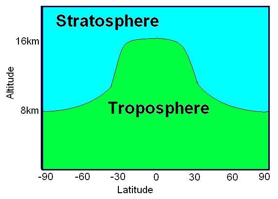
In large part, the earth's ozone distribution is controlled by the properties of the solar-earth system. First, the earth's gravity forces the air to stay around the surface of the earth and form the atmosphere. Second, the sun's energy, directly or indirectly, hits and heats the atmosphere and ground, then radiates away to outer space. Consequently, the atmosphere is stratified into several layers according to the variation in temperature. Meanwhile, UV energy from sunlight enables large-scale atmospheric chemical reactions, including the production and decomposition of ozone molecules. Due to the shape and rotation of the earth and the energy from the sun, there is variability in air pressure. Consequently, diverse air streams transport the products of the atmospheric chemical reactions globally from one place to another. Since the majority of atmospheric ozone is the result of photochemical reactions driven by the energy of the sun, the ozone distribution is dynamically and chemically determined by these processes. Figure 1 shows a plot of the two-dimensional distribution of the monthly mean total column ozone (TCO) in Dobson Units (DU) for the month of October 1988.

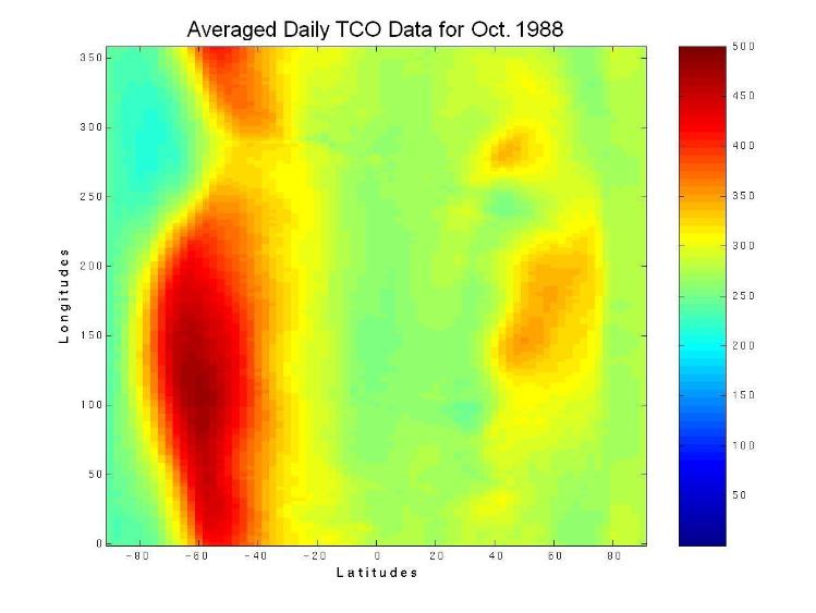
Figure 1. The spatial distribution of averaged daily total column ozone (TCO) data in Dobson Units (DU) for the month of October, 1988. The monthly averaged TCO data came from the British Atmospheric Data Centre (BADC).

From Figure 1, we can see that the highest TCO values are distributed in the mid-latitude regions (particularly in the southern hemisphere), but not in the equatorial or polar regions. To understand this phenomenon, we need to track the lifespan of the atmospheric ozone molecules from birth to death. Chemically, we can explain the procedures with the theory of the Chapman cycle for ozone loss.

Oxygen is one of the crucial constituents of the atmosphere, most of which is free oxygen (O₂). When sunlight enters the atmosphere, atomic oxygen results from the decomposition of O₂ caused by high-energy ultraviolet photons (with wavelengths l shorter than 242 nm):

\begin{align}O_2 \xrightarrow{ \quad hc/ \lambda \quad } O + O\end{align}

where h is Planck's constant, c is the speed of light, and l is the wavelength of the photon (1 nm=10^-9 meters). The oxygen atoms are extremely reactive and can react quickly with oxygen molecules to produce ozone (O₃):

\begin{align}O_2 + O \xrightarrow{ \quad M \quad } O_3\end{align}

where M represents any other molecules that help carry out the reaction and take away the resulting thermal energy. Subsequently, ozone strongly absorbs UV radiation and can reconstitute free oxygen via

\begin{align}O_3 \xrightarrow{ \quad hc/ \lambda \quad } O_2 + O\end{align}

Such kinds of reactions occur so rapidly that the average lifetime of atomic oxygen is less than 1 second, and about 97-99% of the sun's high-frequency light, with wavelengths between 150 and 300nm, are absorbed by the oxygen and ozone molecules. The cycle of chemical reactions achieves a balance through the ozone-loss reaction:

\begin{align}O_3 +  O_3 \xrightarrow{ \quad   \quad } O_2 + O_2 + Q_2\end{align}

Although the global mass of ozone is relatively constant at about 3 trillion kilograms, about 12 percent of the ozone layer is replaced in any single day.

The Chapman cycle theory gives a chemical explanation of the ozone balance in the atmosphere. However, for any given latitude, longitude, and altitude, the ozone concentration is determined not only by the chemical reactions but also by the transport mechanism.

Ozone transportation in the atmosphere is a collateral phenomenon of atmospheric dynamics, which is dominated by atmospheric energy dissipation. Standing on the earth, we can feel the warmth and see the light from the sun above. At an altitude of more than 50km, the air becomes very thin, and this part of the atmosphere contains only a small amount of ozone. Table 1 shows the air pressure at different altitudes. Air pressure is proportional to the air density and it decreases exponentially as a function of altitude: at 8 km it is approximately 300 millibars (mb), at 25km it is approximately 28mb, and at 50km it is approximately 0.9mb.

Table 1. UGAMP Ozone Climatology vertical grid (from the BADC website)

Most high-frequency energy (with wavelengths between 150-300nm) is absorbed in the atmosphere between altitudes of 20km and 50 km via the Chapman cycle. From reaction (2), we know that the M term receives the thermal energy from production of the ozone molecule. Therefore, the results of the Chapman cycle are twofold. One is to replenish the atmosphere with ozone molecules to balance natural ozone loss. The other is to heat the part of the atmosphere where reaction (2) takes place.

On the surface of the earth, thermal effects occur in a different way. Since most high-frequency energy is filtered away by the upper atmosphere, the remaining radiation from the sun cannot support powerful chemical reactions in the lower atmosphere. Instead, the filtered radiation passes through the transparent air and thermally (not chemically) heats the land and sea. Subsequently, the air close to the surface receives thermal energy from the earth by thermal conduction. It is well known that for constant pressure, the warmer the air, the lower its density. Thus, warm air rises and brings the thermal energy upwards by convection. However, the air from the ground can only reach a limited altitude, because the upper air, heated via the Chapman cycle, is warmer and thinner than the lower air. Additionally, the continuous thermal radiation from the earth to outer space ensures the stability of the atmospheric temperature distribution and forms a complete energy dissipative scheme that balances the earth's heating and cooling. As a result of the thermal dynamics, the atmosphere below 50km is stratified into two layers: troposphere (lower layer) and stratosphere (upper layer), and the air between the different layers can only be exchanged rather slowly. Even though a small amount of ozone produced in the stratosphere can enter the troposphere, it will transform back to free oxygen gradually via the Chapman reaction (4). 

Figure 2 shows the separation between the troposphere and the stratosphere as a function of latitude. The morphology of this atmospheric stratification is strongly influenced by the shape of the earth. Since the earth is spherical, the heating effect of the sun is a decreasing function of a location's latitude. In the tropics, the troposphere can achieve higher altitudes, up to 16km. Conversely, in the Antarctic and Artic regions, the thickness of the polar troposphere is only a few kilometers, since the ground temperature is almost always below freezing.

In the troposphere, fierce air convection can quickly blend the air at different altitudes. However, in the stratosphere, because the air is heated from above, it is forced to stay at fixed altitudes. Furthermore, the average UV power from the sun is also a bell-shaped function with its peak at low-latitude regions, again because of the shape of the earth. Although the stratospheric air does not move vertically, the heterogeneous heating, triggered by different seasons and the rotation of the earth, causes numerous strong horizontal air streams that regularly and effectively deliver ozone from the tropical stratosphere to the stratosphere at higher latitudes.

Figure 2. The boundary scheme between the stratosphere and troposphere

Before discussing ozone circulation, we need to go more deeply into the ozone distribution in the atmosphere.

From Figure 1, we see that TCO is approximately a bimodal function of latitude: TCO peaks in the mid-latitude regions and the minimum TCO is in one of the polar regions, depending on the season. Since the tropical stratosphere receives the strongest sunlight, one might have guessed that the maximum TCO is in the low-latitude region, which is contrary to Figure 1. An explanation is given by considering the three-dimensional ozone distribution in the atmosphere.

Figure 3 shows the column-ozone data (in Dobson Units, or DU) averaged over the daily values in October, 1988, for longitude 280E. This plot has the following properties:

1. The column ozone is roughly symmetrically distributed about the equator.
2. Above altitude-level 18 (21.87km), column ozone is a bell-shaped function of latitude with higher values over the tropical region.
3. Between altitude-levels 12 (8.85km) and 18, column ozone is a bimodal function of latitude with the two modes occurring at the mid-latitudes.
4. The delimitation between the lower blue part and the green/yellow/red parts is coincident with the boundary between the stratosphere and the troposphere. (This implies a possible interaction between atmospheric warming and ozone loss. )

The column-ozone distribution is dominated by ozone chemistry and ozone transport action. The ozone transport action is determined by the distribution of the ozone Volume Mixing Ratio (VMR) and atmospheric dynamics. Column ozone and the ozone VMR can be contrasted as follows. For any given column of air, column ozone is proportional to the ozone mass or the number of ozone molecules, but the ozone VMR is the proportion of total volume that is occupied by ozone:

\begin{equation*}VMR \propto \frac{\quad column ozone \quad}{\quad air density \quad}\end{equation*}

Therefore, if column ozone is fixed, ozone VMR is inversely proportional to the air density. And if ozone VMR is fixed, column ozone is proportional to the air density.

Ozone is transported from regions of high ozone VMR to those of low ozone VMR, because the mixing of any two parcels of air equalizes their VMR without changing the total mass of ozone. Therefore, regions of highest ozone VMR are a source of atmospheric ozone, and ozone transportation is implied by the ozone VMR distribution.

Figure 4 shows a typical distribution of ozone VMR in October 1988. The red region and the green/yellow region just above it (between altitudes 26km and 38km) in Figure 4 are where the ozone is generated. The ozone-generating region is above the low latitudes and tropics, which is expected because the strongest UV energy (required for ozone generation) is in this region. Outside of the ozone-generating region, ozone is delivered to higher-latitude regions by horizontal stratospheric air streams. Figure 4 also shows that ozone VMR is a decreasing function of latitude.

Figure 5 shows the ozone VMR plot for January 1988. Compared with Figure 4, the center of the ozone generating region in January 1988 (the Antarctic summer) is shifted a little to the left (south). This phenomenon is the result of the seasonal variation of the solar angle.

In the ozone-generating region, the air density is much smaller than at lower altitudes. As a result, the maximum values of column ozone actually appear at much lower altitude levels. The most plausible way to explain the column ozone distribution is the Brewer-Dobson circulation theory.

Figure 3. The distribution of column ozone (in Dobson Units, or DU) for October 1988 versus latitude and altitude level, for longitude 280E. Each pixel represents the ozone thickness (DU) within the adjacent altitude level at the designated latitude. (The actual altitude of the altitude level can be found in Table 1.)

Figure 4. The distribution of the ozone volume mixing ratio (VMR) in October 1988 for longitude 280E.

Figure 5. The distribution of the ozone volume mixing ratio (VMR) in January 1988 for longitude 280E

The Brewer-Dobson circulation theory states that there is global-scale air circulation in the stratosphere: air rises in low-latitude regions, moves polewards, and then descends, with the largest movement occurring in the winter hemisphere. Many researchers believe that this Brewer-Dobson circulation results from planetary wave (or Rossby wave) events due to the rotation of the earth and the meridional temperature gradients.

From Section 2, we know that the air in the stratosphere has very little vertical movement. In the tropical regions the air rises rather slowly, about 1 meter per hour. (The velocity of the horizontal air stream could be a couple of hundred kilometers per hour.) The air below 16km is almost ozone-free since there is not much ozone in tropospheric air. And 90% of the air at around 16km moves horizontally to the lower-latitude regions before reaching a height of 32km. However, it is between 16km and 32km in the tropical stratosphere where much of the ozone is generated; the rising air brings more and more ozone because of the Chapman reactions (1) and (2).

Beyond the tropical stratosphere, the circulation is polewards at about 30N and 30S, and then gradually descending (Butchart et al., 2002). This phenomenon increases the ozone mass in the mid- and high-latitude regions. In the mid-latitude region, the UV radiation from the sun is not as strong as in the tropics, which weakens the intensity of the Chapman reaction (3) and elongates the lifetime of ozone molecules. When the thinner, high-ozone-VMR tropical stratospheric air moves to the mid-latitude region, the ozone VMR decreases, but the column ozone increases because the air density increases. This theory is consistent with the column ozone distribution shown in Figure 3. Therefore, the Brewer-Dobson circulation theory gives a plausible explanation of the TCO map shown in Figure 1.

The ozone hole is defined as the region where the TCO is below 220 DU, and it occurs in polar regions, usually during the polar winter. Mostly this phenomenon results from the extremely cold polar stratosphere, which causes the formation of the Polar Stratospheric Cloud (PSC). The PSC can convert chlorine to forms that can destroy ozone significantly. See 2002 Ozone-Hole Splitting - Background for more details.

Ozone is important for protecting the earth and organisms living on it from harmful radiation from space. In this exposition, we have attempted to describe the principal factors related to the spatial ozone distribution in the earth's atmosphere.

Daily data on Total Column Ozone (TCO) are collected from remote-sensing satellites and posted on the TOMS website:

The data are highly spatial and achieve global, but non-uniform coverage. Our interest is in mapping daily TCO on a uniform grid of pixels using statistically optimal procedures that also produce variability (i.e., uncertainty) estimates associated with each pixel.

References:

Stratospheric Ozone: An Electronic Textbook. http://www.ccpo.odu.edu/SEES/ozone/oz_class.htm

Butchart, N., Austin J., Knight J. R., and Scaife A. A. (2002). Modeled changes in the stratospheric climate and Brewer-Dobson circulation due to increasing greenhouse-gas concentration. Proceedings of the SPARC 2002 2nd General Assembly of the SPARC/WCRP Project, p/3-4.13