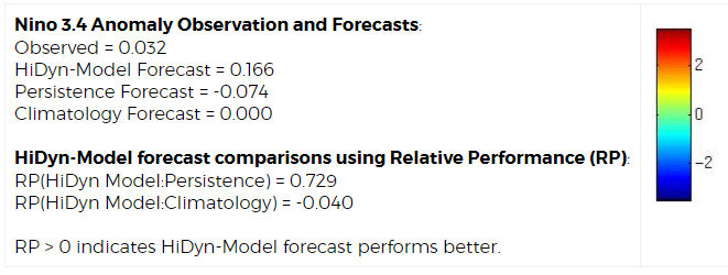
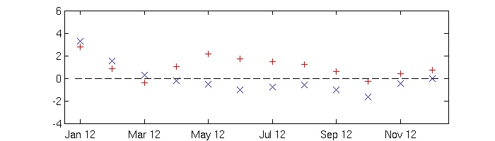
Relative Performance (RP) of HiDyn-Model forecast relative to Persistence forecast (red plus) and to Climatology forecast (blue cross), for 2012 to 2012. RP > 0 indicates HiDyn Model performs better.
SST Forecast Comparisons
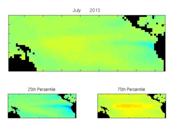
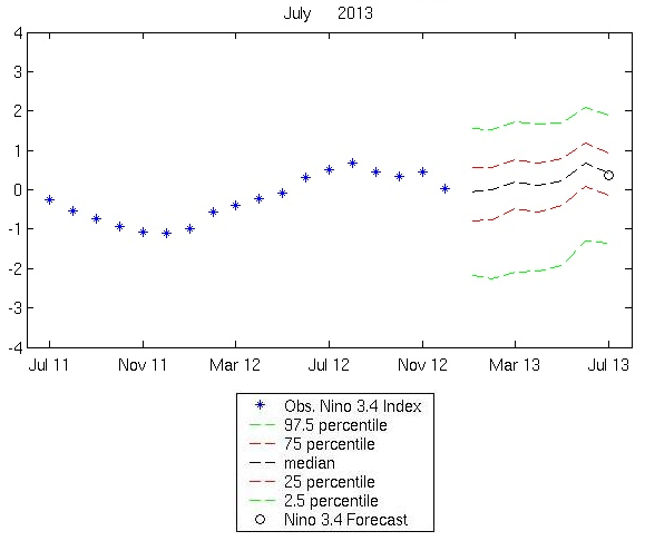
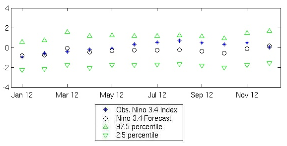
Observed SST anomalies are available for forecast comparisons up to the most recent month of data. HiDyn-Model forecasts for Nino 3.4 anomalies are available from August 1980 up to seven months beyond the most recent month of data. Comparisons are only possible for a selected month for which both the observed ("true") and the forecast SST anomalies are available. A measure of performance of the forecast map is, Performance = ave{(forecast - observed)²}, where the average is taken over all pixels in the Nino 3.4 Region.
Two forecasts, Forecast A and Forecast B, can be compared by the Relative Performance (RP) measure,
RP(A:B) = log(Forecast-B Performance / Forecast-A Performance)
Note that RP(A:B) > 0 indicates that Forecast A performs better than Forecast B.
The HiDyn-Model forecast is compared with two easy-to-compute forecast procedures, namely the Persistence forecast and the Climatology forecast. The Persistence forecast, for a selected month, consists of the observed SST anomalies in the Nino 3.4 Region 7 months earlier. For example, the Persistence forecast for October 1998 consists of the observed anomalies for March 1998. The Climatology forecast is obtained from long-term (typically 30 years) averages of data for each month of the year. Because the data are anomalies, this forecast for any month and any pixel in the Nino 3.4 Region (in fact for any pixel in the Tropical Pacific Region) is 0. Note that to make comparisons of the HiDyn Model's forecasts to another forecast procedure using the RP measure, one must have pixel-level forecasts from the other procedure available in the Nino 3.4 Region.
The performance (or skill) of forecasts can also be compared through their overall correlation with the observed values,
C(A) = corr(Forecast A, Observed),
where
corr = ave{(Forecast A - A*)(Observed - O *)}/{ave(Forecast A - A *)2ave(Observed - O*)2}1/2
and A* = ave(Forecast A) and O* = ave(Observed).
Note that C(A)>C(B) indicates that Forecast A has better performance than Forecast B.
The following table shows C(HiDyn), the correlation coefficient of anomalies of the 7-month-lead HiDyn-Model forecast and C(Persistence), the 7-month-lead Persistence forecast, where the correlations are calculated separately for two 15-year-long periods, 1987-2001 and 1992-2006.
| Model | Years |
|---|
| 1987-2001 |
1992-2006 |
| HiDyn |
0.6543 |
0.6457 |
| Persistence |
0.3597 |
0.2684 |
Correlation coefficients for other ENSO forecast models in the Nino 3.4 Region can be found in van Oldenborgh et al. (2005). The correlation coefficients listed in the table above correspond to a "+6" monthly Nino-3.4 forecast in the terminology of van Oldenborgh et al. (2005). However, they do not go beyond "+5" monthly Nino 3.4 forecasts, so our results and theirs cannot be directly compared.
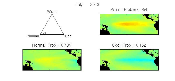
Performance measures based on correlation coefficients have the disadvantage that a forecast could be biased but still have a maximum skill of 1 (a correlation coefficient does not distinguish between forecast=observed and forecast=0.5*observed +1°C). The HiDyn Model is built to forecast well at the 1° × 1° pixel scale in the whole Tropical Pacific Ocean, not just at a regional scale on Nino 3.4. Another skill measure that might be tried is whether the warm/normal/cold regimes of the forecast are correct (These regimes are defined in Berliner et al., 2000). The HiDyn Model should have very high performance in this regard, because of the way it is built.
Reference:
L.M. Berliner, C.K. Wikle, and N. Cressie, 2000. Long-Lead Prediction of Pacific SSTs via Bayesian Dynamic Modeling. Journal of Climate, 13, 3953-3968.
G.J. van Oldenborgh, M.A. Balmaseda, L. Ferranti, T.N. Stockdale, and D.L.T. Anderson, 2005. Did the ECMWF Seasonal Forecast Model Outperform Statistical ENSO Forecast Models over the Last 15 Years? Journal of Climate, 18, 3240-3249.