$ \newcommand{\mb}{\mathbf} \newcommand{\sbf}{\boldsymbol} $

Motivation

Remote sensing data on geophysical variables are almost always indirect measurements of energies received by an instrument that is sensitive to certain bands of the electro-magnetic spectrum. For any one sounding at a given location and time, the result is a several-thousand-dimensional data vector of radiances.

$ \newcommand{\mb}{\mathbf} \newcommand{\sbf}{\boldsymbol} $

Let $\mb{Y}(\mb{s}; t)$ be such a vector of radiances for an atmospheric column from footprint to satellite (e.g., Figure 1), where $\mb{s} = (\text{lon}, \text{lat})$ is the spatial location of the column on the geoid, $D_g \equiv (-180^\circ, +180^\circ)\times(-90^\circ, +90^\circ)$, and $t$ is the time at which the state of the atmospheric column was sensed. Because there are potentially many thousands or millions of radiance vectors for a given time interval, datasets can be very-large-to-massive. In what follows, a statistical approach to remote sensing retrievals and their mapping is given; see Cressie (2018) for more details.

Figure 1: A schematic diagram of the 'A-Train'
satellite constellation showing their respective
remotely sensed atmospheric columns. Image
from http://atrain.nasa.gov/.


Sources of uncertainty

There are a number of sources of uncertainty in spatio-temporal data, including measurement error ("noise"), location error on spatial position, incomplete spatial data in the form of unobserved regions ("missingness"), and spatially overlapping data at several resolutions from possibly different measuring instruments. Spatial fields found in geophysical applications are often subject to dynamical evolution that is strongly governed by physical laws. In many applications, the laws of physics may well be applicable as approximations. Sources of uncertainty in modelling scientific processes include unknown model parameters, unknown initial and/or boundary conditions, unaccounted for fine-scale components, impacts of nonlinearities (e.g., ''chaos''), finite-element approximations, and so forth. Statistical models in space and time have been developed for specific sources of these uncertainties (e.g., Besag, 1974; Ripley, 1981; Cressie, 1993; Chiles and Delfiner, 1999; Banerjee et al., 2004; Le and Zidek, 2006; Lindgren et al., 2011; Cressie and Wikle, 2011; Wikle et al., 2019).

Hierarchical statistical models

Major sources of uncertainty we are interested in are "noise" and "missingness". Statistical remote sensing deals with these and the other uncertainties using statistical models. In our work, we propose the use of hierarchical statistical models (HMs) to predict the true state of the atmospheric column given the retrieved radiances.

The building blocks of HM are a data model, a (scientific) process model, and a parameter model. If $Y$ represents the data, $X$ represents the latent or hidden spatio-temporal process of interest, and $\theta$ represents the parameters, then the data model $[Y|X,\theta]$ allows us to model ''noise'' given the (unknown) process and the parameters; the process model $[X|\theta]$ allows us to model our uncertainty in the scientific process, given the parameters; and the parameter model $[\theta]$ allows us to model our uncertainty in the parameters. Using Bayes rule, we obtain conditional probability distributions for the hidden scientific process given the data, $[X|Y;\theta]$, and hence we can make optimal predictions for $X$ as a function of the data $Y$.

This approach, based on one retrieval at a time, can be used to predict the atmospheric column at each retrieval location. Then, using the predicted state of the atmospheric column as our data, the same approach can be used to ''gap fill'' at locations/times where retrievals are missing. Because of the sheer data size, kriging based on dimension reduction is one possible solution: Fixed Rank Kriging (Cressie and Johannesson, 2008) and Fixed Rank Filtering/Smoothing (Cressie et al., 2010; Katzfuss and Cressie, 2011), along with Spatial Statistical Data Fusion (Nguyen et al., 2012) use spatial and spatio-temporal dependence of the retrieved data to obtain global maps along with a map of the kriging standard deviation.


Global carbon cycle

Our research has focussed on atmospheric carbon dioxide, which is a very important compartment of the global carbon cycle. It is there that its effect as a leading greenhouse gas has been felt. The global carbon cycle describes where carbon is stored and the movement of carbon between these reservoirs (e.g., Figure 2). The oceans and vegetation/soil are examples of CO$_2$ sinks, and fires and anthropogenic emissions are examples of CO$_2$ sources; of the approximately 8 GtC (gigatonnes of carbon) per year that enters the atmosphere, about half is anthropogenic. About 4 GtC stays in the atmosphere, and the other 4 GtC is absorbed roughly equally by oceans and terrestrial processes. This global increase of approximately 4 GtC of atmospheric CO$_2$ per year results in increases in global temperature, and it is unsustainable in the long term.

Figure 2. Simplified schematic of the global carbon cycle. Numbers represent 'carbon stocks' in GtC (1 GtC = 10$^{15}$ gC) and annual carbon exchange fluxes (in GtC yr$^{-1}$). Note that 1 Petagram (Pg) = 1 Gigatonne (Gt). Black numbers and arrows indicate carbon stocks and exchange fluxes estimated for the time prior to the Industrial Era, about 1750. Image from IPCC 5th Assessment Report, Figure 6.1.

It is of paramount importance to be able to characterise precisely where and when carbon sinks and sources occur. Because of a historical lack of extremely precise and very densely sampled CO22 data, these are not very well known. There are several remote sensing instruments that have observation campaigns to measure atmospheric CO22, such as NASA's AIRS instrument and the Japanese space agency's GOSAT instrument.

In July 2014, NASA launched a new instrument, OCO-2, with sensitivity in the lower atmosphere and a very small footprint, allowing fine-spatial-resolution predictions. One negative consequence of a small footprint is that it is harder to capture short-term temporal (i.e., daily) variability, since its high spatial resolution results in a 16-day repeat cycle.

Atmospheric carbon dioxide

There are a number of observational programs that measure atmospheric carbon dioxide (CO2), a leading greenhouse gas. Some of these are land-based and are spatially sparse but temporally rich. Satellite observations solve the spatial-sparseness problem while giving up some temporal richness. The ultimate goal is to use these remote sensing data, which typically represent spatio-temporal column averages of CO2 (in ppm) from Earth's surface to the satellite, to solve the inverse problem of estimating surface CO2 fluxes. This is key, since state-of-the-art climate models (or earth system models) now include an interactive carbon cycle. The most recent satellite launched to measure CO2 is NASA's Orbiting Carbon Observatory-2. Uncertainty quantification starts with the retrieved radiances at individual soundings, progresses to dynamical spatial modelling of column-averaged CO2, and finishes with spatially resolved flux fields. This quantification is crucial to understanding the uncertainties in projected climate, and gives us the ability to see for which regions climate change will be real.

Spatio-temporal HMs

Although the atmosphere mixes rapidly (compared to the oceans), its CO$_2$ concentration is far from homogeneous, and there is a lot of spatio-temporal variability to be accounted for. Hence, it makes sense to write atmospheric CO$_2$ as a spatio-temporal process, $X_{CO2}(\mb{s}; t)$, where $\mb{s}$ ranges over $(\text{lon}, \text{lat})$ and a third dimension, geopotential height $h$, in the spatial domain $D_s$ ($D_s$ is the extent of the atmosphere around the globe); and $t$ ranges over the temporal domain $D_t$ (e.g., $t$ might index days in a given month or weeks in a given season). $X_{CO2}(\mb{s}; t)$ cannot be observed directly. Instead, remote-sensing radiance measurements $\mb{Y}(\mb{s}; t)$ are used to infer the (hidden) state of the atmosphere $\mb{X}(\mb{s}; t)$, from which $X_{CO2}(\mb{s}; t)$ is subsequently predicted. The hierarchical model is

\begin{equation} \mb{Y} = \mb{F}(\mb{X}) + \sbf{\epsilon} \label{FwdFn}, \end{equation}

where $\mb{F}(\cdot)$ is the forward function that relates the hidden multivariate random state $\mb{X}$ to the measured radiance vector $\mb{Y},$ and for clarity we have dropped dependence of $\mb{Y}$ and $\mb{X}$ on $\mb{s}$ and $t$. Our goal is to obtain the predictive distribution of the spatial random field $X_{CO2}(\mb{s};t)$, from which a flux field could be obtained, given all the successfully retrieved OCO-2 data.

The forward function

Consider a single vector of radiances, $\mb{Y}$, for location $\mb{s}$ at time $t$, obtained from a remote-sensing satellite such as the OCO-2 satellite. Each OCO-2 retrieval comprises a large number, $N=3048$, of sensor-based radiance measurements $\mb{Y}=(y_1, ..., y_N)'$ for a set of wavenumbers $\{\nu_i: i=1,...,N\}$ chosen from three regions of the spectrum: The strong CO$_2$ band (4810 - 4897 cm${}^{-1}$), the weak CO$_2$ band (6170 - 6270 cm${}^{-1}$), and the O$_2$ A-band (12950 - 13190 cm${}^{-1}$); see Figure 3 for an example of radiance measurements from these bands.

The purpose of the retrieval is to obtain predictions for the column-averaged CO$_2$ dry air mole fraction in units of parts per million (ppm), $X_{CO2}(\mb{s};t),$ for location $\mb{s}$ at time $t$. Hence the $N$-dimensional OCO-2 radiance vector, $\mb{Y}$, is used to infer relatively few, $n\approx45$, state variables, $\mb{X}=(X_1,...,X_n)',$ that include CO$_2$ dry air mole fraction for a set of vertical levels in the atmosphere, and from which $X_{CO2}(\mb{s};t)$ is obtained. The state vector also includes measures of temperature, pressure, aerosol shape parameters, albedo, and surface wind speed.

The forward function, $\mb{F}(\cdot),$ that relates $\mb{X}$ to the observed radiances, $\mb{Y},$ is a highly complex, deterministic function that quantifies the physical relationship between CO$_2,$ the electro-magnetic radiation that it emits, and the electro-magnetic radiation detected by the satellite as a function of wavelength. The complexity of $\mb{F}(\cdot)$ is illustrated by considering the range of factors that it must include to respect the physics. The algorithm accounts inter alia for the relative geometries of the earth and the sun in relation to the satellite; the solar flux at the top of the atmosphere; Earth's reflectance at the point of measurement; the characteristics of the measuring spectrometer; the state of the atmosphere when the sounding is taken (e.g., the temperature, pressure, and presence of aerosols in the atmosphere); the absorption, emission, and scattering characteristics of the airborne particles whose radiances are being retrieved (and other particles that emit radiation at the same wavelengths), and the interaction of these characteristics with the measuring instrument. As many of the variables in the state vector are used to quantify the flow of energy in the atmosphere (e.g., Figure 4), they are needed in the radiative-transfer-equation-component of the forward function to infer $X_{CO2}(\mb{s};t)$. In practice, approximations to the forward function are made, resulting in a simplified $\mb{F}(\cdot)$ that we shall call the forward model.

The theoretical basis for the retrieval algorithm that is used to predict $X_{CO2}(\mb{s};t)$ from OCO-2 radiance measurements is detailed in the NASA Level 2 Full Physics Retrieval ATBD, which can be found here. Many of the parameter values that are used to calculate the radiance at wavenumber $\nu_i$, are obtained via experiments and recorded in the HITRAN2012 database (e.g., see Rothman et al., 2013).

Figure 3: An example of a retrieval from the OCO-2 satellite. Image source


Figure 4. Global energy flows in the atmosphere. The radiances observed by satellites are used to model a snapshot of these flows from which atmospheric CO$_2$ concentration can be inferred. Image Trenbeth et al. (2009) Figure 1.

State vector prediction

Making inference on $\mb{X}$ is a challenging statistical problem. State-vector predictions are obtained by solving the ''inverse problem'' for \eqref{FwdFn} using the observed radiances. However, as $\mb{F}(\cdot)$ is non-linear and there is noise in the data (along with uncertainty in the a-priori distribution of the state variables), multiple values of the state variables may produce the same observed radiances; linear statistical methods cannot be used, and an analytical solution to the problem is not possible. A state-space approach, that numerically minimises a cost function $\mb{J}$, is used to solve the inverse problem, where $\mb{J}$ consists of a fidelity-to-the-data term and a prior-information term; see \eqref{inverseEqn} below.

Numerical approaches to solving the inverse problem include those based on Twomey-Tikhonov regularisation (see Doicu et al, 2010, for a recent review). Statistical approaches include ridge regression, penalised likelihood, and Bayesian posterior analysis (e.g., Cressie and Wang, 2013, and the references therein). Each of these approaches uses a form of optimal estimation (e.g., Rodgers, 2000) to obtain a predictor, $\hat{\mb{X}}(\mb{y})$ of $\mb{X}$, by iteratively minimising the cost function, \begin{align} \mb{J} = (\mb{y} - \mb{F}(\mb{X}))' \sbf{\Sigma}_\epsilon^{-1} (\mb{y} - \mb{F}(\mb{X})) + (\mb{X} - \mb{X}_a)' \sbf{\Sigma}_a^{-1} (\mb{X} - \mb{X}_a), \label{inverseEqn} \end{align}

where $\mb{Y}=\mb{y}$ are the observed radiances. This results in predictions, $\hat{\mb{X}}(\mb{y})$, of the state $\mb{X}$ (e.g., Connor et al., 2008; O'Dell et al., 2012; Crisp et al., 2014). In a final step, the measures of CO$_2$ dry air mole fraction in the state vector are combined to obtain a prediction, $\hat{X}_{CO2}(\mb{s};t)$, for $X_{CO2}(\mb{s};t)$, for location $\mb{s}$ at time $t$.

Spatial prediction

Due to the constraints of satellite orbits and viewing angles and the presence of aerosols in the atmosphere, the number of retrievals for which $X_{CO2}(\mb{s};t)$ can be predicted is typically sparse for a given orbit of the earth; see Figure 5 for an example of the global distribution of OCO-2 retrievals. We use a statistical model to smooth the data, $\hat{X}_{CO2}(\mb{s};t),$ in order to predict $X_{CO2}(\mb{s};t)$ at locations where data are missing, and to create global maps of $\hat{X}_{CO2}(\mb{s};t)$ at time $t$, such as the one shown in Figure 6. One of the most popular statistical models for spatial/spatio-temporal datasets is the Spatial Mixed Effect (SME) model (Cressie and Johannesson, 2008).

Figure 5: Averaged CO2 concentrations from OCO-2 for the period 21 November - 29 December, 2014. 
Image from http://disc.sci.gsfc.nasa.gov/datareleases/First_CO2_data_from_OCO-2.

To predict $X_{CO2}(\mb{s};t)$ for a location $\mb{s}_0$ at time $t_0,$ for which a retrieval is missing, we use the $m$ successfully retrieved CO$_2$ concentrations, $\mb{X}^P = (\hat{X}_{CO2}(\mb{s}_1;t_1), ..., \hat{X}_{CO2}(\mb{s}_m;t_m))'$ as our data. In the following paragraphs, we omit the time coordinate $t$ to focus on the purely spatial case, $X_{CO2}(\mb{s})$; $\mb{s}\in D_g$.

It is assumed that $\hat{X}_{CO2}(\mb{s}_i)$ is unbiased for $X_{CO2}(\mb{s}_i)$ and $\mathrm{var}(\mb{X}^P)\equiv \mb{\Sigma}_{\varepsilon}$. We model the true spatial random field $X_{CO2}(\cdot)$, using an SME model, \begin{eqnarray*} X_{CO2}(\mb{s})=\mb{Z}(\mb{s})'\sbf{\beta}+\nu(\mb{s})+\xi(\mb{s});\mb{s}\in D_g, \end{eqnarray*} where $\mb{Z}(\cdot)'\sbf{\beta}$ describes the spatial trend with $p$ covariates $\mb{Z}(\mb{s})=(Z_1(\mb{s}), \ldots, Z_p(\mb{s}))',$ and the small-scale dependence, $\nu(\mb{s}),$ is modelled using a Gaussian spatial process, $\nu(\cdot)=\mb{S}(\cdot)'\sbf{\eta}$, that follows a Spatial Random Effect (SRE) model (Cressie and Johannesson, 2008). That is, $\mb{S}(\cdot)=(S_1(\cdot),\ldots, S_r(\cdot))'$ is an $r$-dimensional vector of multi-resolution basis functions, and $\sbf{\eta}$ is an $r$-dimensional random vector with a mean of zero and an unknown covariance matrix, $\mb{K}$. The last term, $\xi(\mb{s}),$ is a process that is used to model fine-scale variability. It has a mean of zero and $\sbf{\xi} = (\xi_1, \ldots, \xi_m)'$ has a covariance matrix $\sbf{\Sigma}_\xi$ that we have assumed is a diagonal matrix with constant variance, $\sigma^2_\xi$. To ensure the identifiability of $\xi(\cdot),$ we also assume that $\sbf{\Sigma}_\varepsilon$ is known.

The SRE model has two merits for modelling large spatial datasets.

  • It performs dimension-reduction of the underlying smooth spatial process $\nu(\cdot)$ so that the SRE model has the capacity for modelling datasets of a massive size. If the number of basis functions $r$ is chosen to be small, the resulting covariance matrix of $\nu(\cdot)$ is of low rank. Consequently, the likelihood can be efficiently evaluated; see Cressie and Johanneson (2008).
  • Multi-resolution basis functions, $\mb{S}(\cdot)$, with basis centres covering the entire spatial domain are capable of capturing the non-stationary nature of the dataset.

Estimation of the unknown covariance matrix $\mb{K}$ is a crucial step in obtaining predictions of $X_{CO2}(\mb{s})$ from the SME model. There are several parameter estimation methods available for estimating $\mb{K}$, such as the Method of Moments (Cressie and Johannesson, 2008), the Expectation-Maximization algorithm (Katzfuss and Cressie, 2011) and a Bayesian approach to inference based on Givens-angle priors (Kang and Cressie, 2011). Estimation of $\sigma^2_{\xi}$ is done in conjunction with that of $\mb{K}$.

After we obtain estimates $\tilde{\mb{K}}$ and $\tilde{\sigma}^2_\xi$, empirical optimal spatial prediction for predictive locations $\mb{s}_0$ is performed using Fixed Rank Kriging (FRK). The optimal predictor, $\tilde{X}_{CO2}(\mb{s}_0),$ of $X_{CO2}(\mb{s}_0)$ under the SME model is given by, \begin{eqnarray*} \tilde{X}_{CO2}(\mb{s}_0)=\mb{Z}(\mb{s}_0)'\tilde{\sbf{\beta}}+\tilde{\mb{k}}(\mb{s}_0)'\mb{\Sigma}_{\mb{x}}^{-1}(\mb{X}^P - \mb{Z}\tilde{\sbf{\beta}}), \end{eqnarray*} where $\tilde{\sbf{\beta}} =(\mb{Z}'\mb{\Sigma}_{\mb{x}}^{-1}\mb{Z})^{-1} \mb{Z}' \mb{\Sigma}_{\mb{x}}^{-1} \mb{X}^P$ is the generalised-least-squares estimate of the spatial-trend parameters $\sbf{\beta},$ $\mb{\Sigma}_{\mb{x}}\equiv(\mb{S}\tilde{\mb{K}}\mb{S}' + \tilde{\sigma}^2_{\xi}\mb{I}_m + \mb{\Sigma}_{\varepsilon})$ is the covariance matrix for the retrieved CO$_2$ concentrations, and $\tilde{\mb{k}}(\mb{s}_0)=\mb{S}(\mb{s}_0)'\tilde{\mb{K}}\mb{S}'$ is the correlation between $X_{CO2}(\mb{s}_0)$ and $\mb{X}^P$. The computational complexity of the inverse operation, $\mb{\Sigma}_{\mb{x}}^{-1}$, is linear in $m$ when the Sherman-Woodbury-Morrison inversion formula is used, so the FRK predictor can be efficiently applied where there are a very large number of prediction locations.

An example of a map of predicted CO$_2$ concentrations obtained using retrievals from the OCO-2 satellite is shown in Figure 6. A kriging predictor was used to obtain the spatial predictions used in this map.

Figure 6: Global atmospheric carbon dioxide concentrations for the period 1 October - 11 November, 2014, as recorded by NASA's Orbiting Carbon Observatory-2. NASA/JPL-Caltech. Image from http://www.nasa.gov/jpl/oco2/pia18934.


Banerjee, S., Carlin, B. P., and Gelfand, A. E. (2004). Hierarchical Modeling and Analysis for Spatial Data. Chapman & Hall/CRC Press, Boca Raton, FL.

Besag, J. (1974). Spatial interaction and the statistical analysis of lattice systems, Journal of the Royal Statistical Society, Series B, 36, 192-236.

Chiles, J.-P. and Delfiner, P., (1999). Geostatistics: Modelling Spatial Uncertainty. Wiley, New York, NY.

Connor, B. J., Bosch, H., Toon, G., Sen, B., Miller, C. and Crisp, D. (2008). Orbiting Carbon Observatory: Inverse method and prospective error analysis. Journal of Geophysical Research: Atmospheres, 113, 1-14.

Cressie, N. (1993). Statistics for Spatial Data (revised edition). Wiley, New York, NY.

Cressie, N. (2018). Mission CO2ntrol: A statistical scientist’s role in remote sensing of atmospheric carbon dioxide, (with discussion). Journal of the American Statistical Association, 113, 152-181.

Cressie, N. and Johannesson, G. (2008). Fixed rank kriging for very large spatial data sets. Journal of the Royal Statistical Society, Series B, 70, 209-226.

Cressie, N., Shi, T., and Kang, E. L. (2010). Fixed rank filtering for spatio-temporal data. Journal of Computational and Graphical Statistics, 19, 724-745.

Cressie, N. and Wang, R. (2013), Statistical properties of the state obtained by solving a nonlinear multivariate inverse problem. Applied Stochastic Models in Business and Industry, 29, 424-438.

Cressie, N. and Wikle, C. K. (2011). Statistics for Spatio-Temporal Data. Wiley, Hoboken, NJ.

Crisp, D., Fisher, B. M., O'Dell, C., Frankenberg, C., Basilio, R., Bosch, H., Brown, L. R., Castano, R., Connor, B., Deutscher, N. M., Eldering, A., Griffith, D., Gunson, M., Kuze, A., Mandrake, L., McDuffie, J., Messerschmidt, J., Miller, C. E., Morino, I., Natraj, V., Notholt, J., O'Brien, D. M., Oyafuso, F., Polonsky, I., Robinson, J., Salawitch, R., Sherlock, V., Smyth, M., Suto, H., Taylor, T. E., Thompson, D. R., Wennberg, P. O., Wunch, D. and Yung, Y. L. (2012). The ACOS CO2 retrieval algorithm - Part II: Global XCO2 data characterization. Atmospheric Measurement Techniques, 5, 687-707.

Doicu, A., Trautmann, T., and Schreier, F. (2010). Numerical Regularization for Atmospheric Inverse Problems. Springer, Berlin.

O'Dell, C. W., Connor, B., Bosch, H., O'Brien, D., Frankenberg, C., Castano, R., Christi, M., Eldering, D., Fisher, B., Gunson, M., McDuffie, J., Miller, C. E., Natraj, V., Oyafuso, F., Polonsky, I., Smyth, M., Taylor, T., Toon, G. C., Wennberg, P. O. and Wunch, D. (2012). The ACOS CO2 retrieval algorithm - Part 1: Description and validation against synthetic observations. Atmospheric Measurement Techniques, 5, 99-121.

Kang, E. and Cressie, N. (2011). Bayesian Inference for the Spatial Random Effects Model. Journal of the American Statistical Association, 106, 972-983.

Katzfuss, M. and Cressie, N. (2011). Spatio-temporal smoothing and EM estimation for massive remote-sensing data sets. Journal of Time Series Analysis, 32, 430-446.

Le, N. D., and Zidek, J. V. (2006). Statistical Analysis of Environmental Space-Time Processes. Springer, New York, NY.

Lindgren, F., Rue, H., and Lindstrom, J. (2011). An explicit link between Gaussian fields and Gaussian Markov random fields: The stochastic partial differential equation approach (with discussion). Journal of the Royal Statistical Society, Series B, 73, 423-498.

Nguyen H., Cressie N., Braverman A. (2012). Spatial statistical data fusion for remote sensing applications. Journal of the American Statistical Association, 107, 1004-1018.

Ripley, B. D. (1981). Spatial Statistics. Wiley, New York, NY.

Rodgers, C. D. (2000). Inverse Methods for Atmospheric Sounding: Theory and Practice. World Scientific, Singapore.

Rothman, L. S., Gordon, I. E., Babikov, Y., Barbe, A., Chris Benner, D., Bernath, P. F., Birk, M., Bizzocchi, L., Boudon, V., Brown, L. R., Campargue, A., Chance, K., Cohen, E. A., Coudert, L. H., Devi, V. M., Drouin, B. J., Fayt, A., Flaud, J. M., Gamache, R. R., Harrison, J. J., Hartmann, J. M., Hill, C., Hodges, J. T., Jacquemart, D., Jolly, A., Lamouroux, J., Le Roy, R. J., Li, G., Long, D. A., Lyulin, O. M., Mackie, C. J., Massie, S. T., Mikhailenko, S. , Muller, H. , Naumenko, O. V., Nikitin, A. V., Orphal, J., Perevalov, V., Perrin, A., Polovtseva, E. R., Richard, C. , Smith, M., Starikova, E., Sung, K., Tashkun, S., Tennyson, J., Toon, G. C., Tyuterev, V. and Wagner, G. (2013). The HITRAN2012 molecular spectroscopic database. Journal of Quantitative Spectroscopy and Radiative Transfer, 130, 4-50.

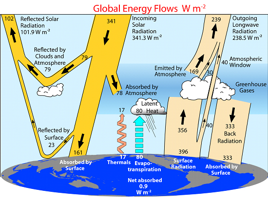
Trenberth, K. E., Fasullo, J. T., and Kiehl, J., (2009). Earth's global energy budget. Bulletin of the American Meteorological Society, 90, 311-323.

Wikle, C. K., Zammit-Mangion, A., and Cressie, N. (2019). Spatio-Temporal Statistics with R. Chapman and Hall/CRC Press, Boca Raton, FL.


Authored by N. Cressie, A. Burden, and B. Zhang, 2015; revised  2020.