Regional flux inversion
Methane is one of the most prevalent greenhouse gases emitted, second only to CO2 in the UK. It is has a shorter lifetime in the atmosphere than CO2, but it does a much better job at trapping heat. Many countries are trying to reduce methane emissions, and hence their government bodies and agencies need constantly updated flux estimates. This is usually done 'bottom-up,' using inventories (built from expert knowledge and scientific trials) that incorporate within them the expected methane fluxes from a region given its current characteristics (e.g., percentage farmland). See Figure 1 for the inventory EDGAR.
Another, arguably more direct way to obtain flux estimates is to use observational data of methane mole fraction obtained at certain locations in time and space. There are several stations in the UK designed to record methane (we use four in this study). Mole fraction is not a direct indicator of methane flux, since the methane particles are transported around, sometimes over great distances, before they are detected. To know from where the methane particles have emanated, a transport model is generally employed, which uses meteorological information to trace back the trajectory of the particles in time. These so-called Lagrangian particle dispersion models (LPDMs) are complex computer programs that are highly compute-intensive. The one we used in this study is the Numeric Atmospheric-dispersion Modelling Environment (NAME), more details of which can be found on the Met Office website here. The question then is, how do we incorporate a model like NAME with observations at a few locations in order to estimate (methane) gas fluxes? The answer to this question has resulted in what is now a scientific field in its own right known as 'atmospheric trace-gas inversion'. As we discuss next, there are some limitations to current state-of-the-art trace-gas inversion techniques that we believe spatio-temporal statistics can help overcome.
Work presented on this page is joint with researchers at the University of Bristol, UK and the MetOffice in Exeter, UK.
Figure 1: The emissions database for global atmospheric research (EDGAR). Source: http://edgar.jrc.ec.europa.eu/
Conventional model
Let the mole-fraction observation at location $\s$ and time $t$ be denoted as $Z_{m,t}(\svec)$, and define $D_{m,t}^O$ as the set of measurement locations at time $t$. Further, denote the collection of all observation locations as $D^O_m \equiv \bigcup_{t \in \mathcal{T}} D^O_{m,t}$, where $\mathcal{T} \equiv \{1,\dots,T\}$ is the temporal domain, and $T > 1$ is the number of time steps. There are typically very few or no direct observations on fluxes; flux prediction usually proceeds by using the following univariate model (or its discretised equivalent) for inversion \begin{equation}\label{eq:uv} Z_{m,t}(\svec) = \int_D b_t(\svec,\uvec)Y_f(\uvec)\intd\u + e_{m,t}(\svec); \quad \svec \in D^O_{m,t};\quad t \in \mathcal{T}, \end{equation} where $D$ is the spatial domain, $e_{m,t}(\svec)$ is (Gaussian) observation error, $b_t(\svec,\uvec)$ is the interaction function, or source-receptor relationship (SRR) obtained from NAME that returns quantities with dimension [time][mass]$^{-1}\hspace{-0.05in}$, and $Y_f(\cdot)$ is the flux field that returns quantities with dimension [mass][time]$^{-1}$[area]$^{-1}\hspace{-0.05in}$. The field $Y_f(\cdot)$ is a stochastic process with statistical properties that reflect those of the underlying process (e.g., positivity). Note that there is no mention of the whole mole-fraction field, only observations of the mole-fraction field at specific locations.
The limitations of this conventional model stem from the following:
- Often, Gaussianity (or truncated-Gaussianity) of $Y_f(\cdot)$ is assumed, even though this is rarely the case in reality. There are very few sinks of methane, and a histogram of fluxes from inventories indicates that its distribution is highly skewed. Generally, Gaussianity is not a valid assumption for methane.
- Of those works that allow for deviation from Gaussianity, none assumes spatial correlation. We believe that borrowing of strength spatially can greatly improve predictions. Simple visualisation of the flux maps (e.g., Figure 1) reveals that spatial correlation is indeed present.
- The above model \eqref{eq:uv} lumps together error due to measurement and error due to the SRR. This is a questionable simplification, since the statistical properties of these two error terms are very different from one another. This may be remedied by using a latent mole-fraction field in \eqref{eq:uv} and then linking the mole-fraction observations to this.
We propose the following model to address all of these concerns.
Proposed model
We assume a bivariate spatial model, where the first variate is the flux and the second variate is the mole fraction. With our model, the object of interest shifts from the observations of mole fraction to the mole-fraction field itself, which we model as \begin{equation}\label{eq:mv} Y_{m,t}(\svec) = \int_D b_t(\svec,\uvec)Y_f(\uvec)\intd\u + \zeta_{t}(\svec); \quad \svec \in D^L_m;\quad t \in \mathcal{T}, \end{equation} where $Y_{m,t}(\cdot)$ is the mole-fraction field and $D^L_m$ is a user-defined set of discrete locations in $D$ at which $Y_{m,t}$ is evaluated. The additive component, $\zeta_{t}(\svec)$, captures the spatio-temporal offset (due to mole-fraction background) and variation in the true mole-fraction field that cannot be explained by the flux field through the SRR. Note that $\zeta_{t}(\svec)$ is different from $e_{m,t}(\svec)$ in \eqref{eq:uv}, since it explicitly accounts for SRR misspecification. Finally, the observations available for the inversion are not the field itself, but a noisy, incomplete version of it: \begin{equation}\label{eq:obs} Z_{m,t}(\svec) = Y_{m,t}(\svec) + \varepsilon_{m,t}(\svec); \quad \svec \in D^O_{m,t}, \end{equation} where $\varepsilon_{m,t}(\cdot)$ is a measurement-error process.
There are three important differences between \eqref{eq:uv} and \eqref{eq:mv}. First, \eqref{eq:mv} is defined on $D^L_m$, whereas \eqref{eq:uv} is only defined for $D_{m,t}^O \subset D$. Hence, in our proposed model, the locations at which mole fraction is inferred need not coincide with the observation locations. Putting $D^L_m = D_m^O$ is only one special case. Second, due to the decoupling, the locations $\svec \in D^L_m$ at which the SRR is evaluated are not dependent on the observation locations; the case of $|D^L_m| \ll |D^O_m|$ is important for regional studies that use computationally intensive LPDMs to simulate the SRR: In the model based on \eqref{eq:uv}, the SRR needs to be evaluated for each location in $D^O_m$, while in the bivariate model the SRR needs to be evaluated for each location in $D^L_m$. Third, the mole-fraction observations do not appear in \eqref{eq:mv}. This is computationally beneficial as it is usually reasonable to assume that observations are conditionally independent given the mole-fraction field, but not necessarily given only the flux field. This conditional independence implies that the conditional covariance matrix (given the mole-fraction field) of a collection of $Z_{m,t}(\svec)$ is diagonal, resulting in simplified matrix computations.
To date, most studies have assumed either that $Y_f(\cdot)$ is a Gaussian process or that $Y_f(\cdot)$ is spatially uncorrelated and non-Gaussian. As explained above, it is generally important to model non-Gaussianity since the spatial distribution of fluxes tends to exhibit asymmetry with a right heavy tail. Indeed, for some trace gases such as methane, it is reasonable to assume that it has only positive support. Further, it is easy to see from flux inventories that often the spatially uncorrelated assumption is unrealistic. Therefore, to cater for these aspects, we assume that $Y_f(\cdot)$ is a spatial process such that $\widetilde{Y}_f(\cdot) \equiv \ln Y_f(\cdot)$ is a Gaussian process. Then $Y_f(\cdot)$ is termed a lognormal spatial process; clearly, $P(Y_f(\svec) \le 0) = 0$, for $\svec \in D\hspace{-0.03in}$, so that $Y_f(\cdot)$ is (almost surely) positive.
Inference
Atmospheric trace-gas inversion is generally highly computationally intensive, not only because of the large amount of data involved, but also because of the ill-posed nature of the problem. While a unique set of emissions and SRR map to a unique mole-fraction time series (in the absence of discrepancy), the converse is not necessarily the case. We deal with identifiability and computational issues in three ways:
- We estimate parameters in the covariance function describing the flux field from inventory data; that is, we assume that the spatial properties (length scale, roughness, and variance) of the inventory are correct.
- We use an empirical hierarchical model (EHM) for the bivariate field, where the parameters appearing in the SRR discrepancy term are estimated before being plugged in an empirical predictive distribution of the bivariate field. We use an expectation maximisation (EM) algorithm to estimate these parameters. Since the E-step cannot be computed exactly, we carry out Laplace approximations; that is, we replace the first and second moments of the field required at each step with those obtained from a Laplace approximation.
- Since gradient information is readily available we use Hamiltonian Monte Carlo (HMC) in order to construct the empirical predictive distribution (after following plugging-in of the parameter estimates). HMC was chosen after various experiments with Metropolis-Hastings and slice sampling failed.
Results
Following data pre-processing (see paper below for details), we applied our approach to estimate methane flux in the UK and Ireland. The pointwise posterior median and 95th percentile of the methane flux field are shown in the centre and right panel, respectively, of Figure 2, and they should be compared with the inventory emissions map shown in the left panel. We obtain total estimates for the UK and Ireland (including the sea territories) of 2.23 $\pm$ 0.08 Tg yr$^{-1}$ and 0.37 $\pm$ 0.05 Tg yr$^{-1}\hspace{-0.05in}$, respectively. Both these estimates are lower than those obtained from the inventory shown in the left panel (2.65 Tg yr$^{-1}$ and 0.64 Tg yr$^{-1}\hspace{-0.05in}$, respectively), and they support the conclusion in Ganesan et al. (2015) that the methane emissions obtained from the inventory might be too large.
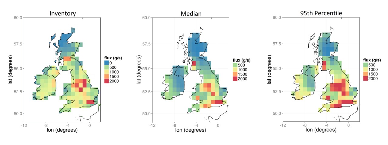
Interestingly, despite the omission of a spatially varying prior distribution, the posterior spatial distribution of emissions is compatible somewhat with that in the inventory. However, there are some key differences. Many large cities, such as Edinburgh, Glasgow, and Dublin, were estimated to have lower methane emissions than those given by the inventory. On the other hand, we obtained larger emissions for the south of the UK, most notably a median total emission of 0.128 Tg yr$^{-1}\hspace{-0.05in}$ in the grid cell containing London, which compares to 0.062 Tg yr$^{-1}\hspace{-0.05in}$ in the inventory. We note that there is no consensus on methane emissions in London (Helfter et al., 2013), but out result supports others that say there is a two- to three-fold difference between inventory and measured fluxes in central London.
In Figure 3, we show the distributions of mole fraction at each station location during the month of January 2014, together with those observations used to train the model (black crosses) and those observations left out for validation (red crosses). The first thing to note is that the distributions of mole fractions are available at times when observations are missing. Mole-fraction uncertainty increases at these times, but clear patterns are also discernible (e.g., at the station RGL, the peak at $t$ =130 is noticeable). It would be straightforward to show the distribution of mole fractions at non-observation locations, however this requires the interaction function to be evaluated at these locations too. Second, sometimes the posterior density of the mole fraction at a space-time coordinate $(\svec,t)$ might have probability mass on the negative real axis. This does not imply a negative (unphysical) mole fraction, rather an imperfect correction of the background, which in this example is on the order of 1900 ppb. Third, the observations used for validation lie within the 90% prediction intervals, with the exception of a few outliers. The ability to obtain what seems to be realistic predictions for out-of-sample mole fractions increases our confidence in inferences for $Y_f(\cdot)$. However, without the availability of validation methane-flux data, critical predictive performance measures in trace-gas inversion cannot be obtained.
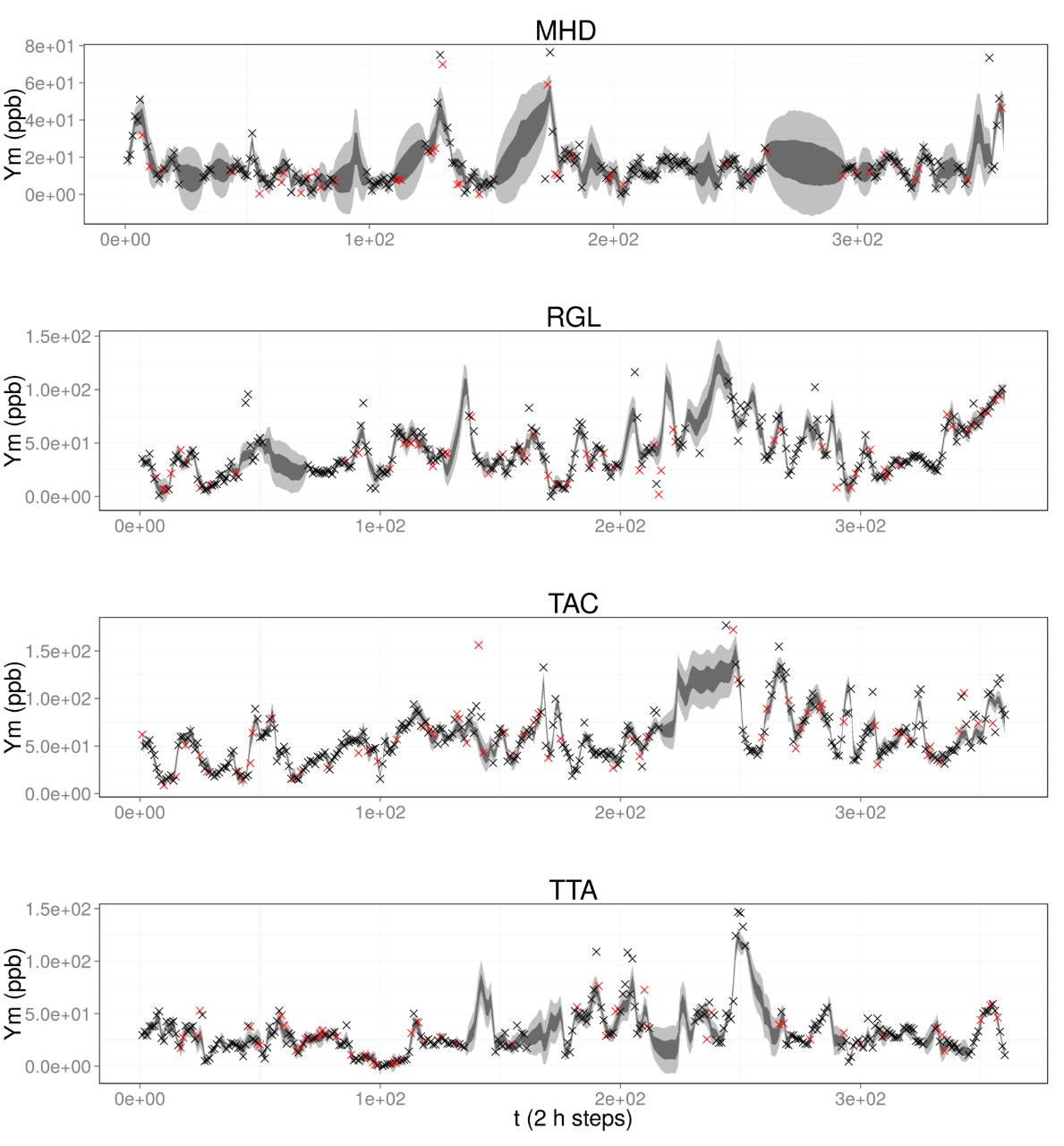
Figure 3: Distributions of mole fraction (with the background mole fraction subtracted) due to UK and Ireland land-based emissions at the four measurement stations (MHD, RGL, TAC, and TTA), where $t = 1$ corresponds to 1 January 2014 00:00, $t = 2$ corresponds to 1 January 2014 02:00, and so on until 31 January 2014 22:00. The dark and light shadings denote the interquartile and the 5th–95th percentile ranges, respectively. The red crosses denote the observations used for validation, whilst the black crosses denote those used for training.
Reproducible code
The code used in this work, that has been packaged and versioned, can be found here.
Publications
The work described here is detailed in the following articles:
C. Helfter, E. Nemitz, J. F. Barlow, C. R. Wood (2013). Carbon dioxide & methane emission dynamics in central London (UK), Poster presented at the EGU General Assembly, Vienna Austria. [Online; accessed 01 March 2015]
A. L. Ganesan, A. J. Manning, A. Grant, D. Young, D. E. Oram, W. T. Sturges, J. B. Moncrie, S. O'Doherty (2015). Quantifying methane and nitrous oxide emissions from the UK using a dense monitoring network, Atmospheric Chemistry and Physics 15, 857–886.
S. M. Miller, S. C. Wofsy, A. M. Michalak, E. A. Kort, A. E. Andrews, S. C. Biraud, E. J. Dlugokencky, J. Eluszkiewicz, M. L. Fischer, G. Janssens-Maenhout, B. R. Miller, J. B. Miller, S. A. Montzka, T. Nehrkorn, C. Sweeney (2013). Anthropogenic emissions of methane in the United States, Proceedings of the National Academy of Sciences 110, 20018–20022.
M. Rigby, A. J. Manning, R. G. Prinn (2011). Inversion of long-lived trace gas emissions using combined Eulerian and Lagrangian chemical transport models, Atmospheric Chemistry and Physics 11, 9887–9898.
Authored by A. Zammit-Mangion and N. Cressie, 2017; revised 2020.